| GISdevelopment.net ---> AARS ---> ACRS 1997 ---> Poster Session 3 |
Determination of Haze from
Satellite Remotely Sensed Data: Some Preliminary Results
Asmala Ahmad and Mazlan
Hashim
Faculty of Engineering and Geoinformation Science
Universiti Teknologi Malaysia
Locked Bag 791, 80990 Johor Bahur
Phone : 07-5502940 Fax : 07-5566163
E-mail : mazland@fksg.utm.my
Abstract Faculty of Engineering and Geoinformation Science
Universiti Teknologi Malaysia
Locked Bag 791, 80990 Johor Bahur
Phone : 07-5502940 Fax : 07-5566163
E-mail : mazland@fksg.utm.my
This paper reports some preliminary results of a study conducted at Centre for Remote Sensing UTM in attempt to quantify haze (total suspended particulates) from NOAA AVHRR data. The relationship between measured total suspended particulates (TSP) and satellite recorded digital number (DN) were analysed. TSP measurements were carried out by Malaysian Meteorological Services at eight air pollution stations located in Peninsular Malaysia. Initial results of this relationship were shown as regression plots namely, linear, logarithmic, polynomial, power and exponential.
Introduction
Haze can be defined as a partially opaque condition of the atmosphere caused by very tiny suspended solid or liquid particulars in the air (Morris, 1975). Haze, related to atmospheric aerosol released from an open burning or forest fire contains large amount of trace gases (e.g., CO2, CO, CH4, Nox) and particulates (e.g., organic matter, graphitic carbon). Haze is hazardous to health, especially associated with lung and eye diseases. Long term haze occurrence will increase the atmospheric greenhouse effects besides affecting the trospheric chemistry. Thus, haze occurrence should be identified so that necessary measures could be taken to curb such occurrence. Conventionally, haze can be determined from ground measurements instruments such as air sampler, sun photometer, and optical particle counter, however these instruments could not detect an early sign of haze and is impractical if measurement are to be made over relatively large areas or for continuous monitoring.
The haze episode occurred during mid-August to October 1994 is considered one of the worst since 1980 (four similar haze episodes had occurred in April 1983, August 1990, June 1991 and October 1991). It was due to the injection of suspended ash particulates from large scale forest fie in Sumatra and Kalimantan. In addition, the occurrence of shallow localized haze in Klang Valley since the past two decades during the South West Monsoon Season (months of July to September) acted as the minor contributor that made the condition worse. Such phenomenon (which was not a new experience for Malaysia) has created moiré awareness among the people concerning the haze problem and more commitment are put to curb haze occurrences effectively.
This paper reports some preliminary results in attempt to quantify haze from NOAA AVHRR data. Initial relationship between TSP and satellite DN were shown at eight air pollution stations namely Bayan Lepas, Petaling Jaya, Perai, Melaka, Kuala Terengganu, Mersing, Endau, Kuantan and Batu Embun.
Materials and Methods
a) Satellite Data
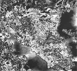
The NOAA 12 AVHRR satellite data dated 30 September 1995 (0657 UTC), which were obtained from the Malaysian Meteorological service were used in this study. The data was subseted to area of interest - The Penisular Malaysia (see Figure 1). Eight air pollution stations measurement of TSP at the day of satellite data acquisatin are shown as Table 1.
| Stations: | |
| 1 Bayan Lepas | 5 Kuala Terengganu |
| 2 Peteling Jaya | 6 Mersing |
| 3 Perai | 7 Kuantan |
| 4 Melaka | 8 Batu Embun |
(b) Total Suspended Particulates (TSP)
The suspended particulates (generally known as aerosols) are minute non-aqueous matter (sizes ranging from 0.1 microns to 100 microns) floating in the atmosphere that will never settle to the ground because their higher buoyancy forces exceed the gravitational pull (Malaysian Meteorological Service, 1995).
The ground measured total suspended particulates (TSP) used in this study are collected from the Malaysian Meteorological Service. The corresponding TSP values at the selected eight air pollution stations are shown in Table 1.
| Air Pollution Station | Geographic Coordinates | Altitude (m) | *Instrument Used | TSP(mgm/m3) | ||
| Latitude | Longitude | |||||
| 1. | Bayan Lepas | 05° 18'N | 100°16'E | 3.3 | HVAS&AAPS | 29 |
| 2. | Petaling Jaya | 03°06'N | 101°39'E | 45.7 | HVAS & APS | 78 |
| 3. | Perai | 05°21'N | 100°24'E | 1.0 | HVAS &AAPS | 164 |
| 4. | Melaka | 02°16'N | 102°15'E | 8.0 | HVAS&ERNI | 43 |
| 5. | Kuala Terengganu | 05°23'N | 103°06'E | 5.0 | HVAS&AAPS | 36 |
| 6. | Mersing | 02°27'N | 103°50'E | 44.0 | HVPM10&APS | 24 |
| 7. | Kuantan | 03°47'N | 103°13'E | 15.3 | HVPM10&APS | 28 |
| 8. | Batu Embun | 03°58'N | 102°21'E | 59.5 | HVPM10&APS | 26 |
*Note
HVPM : High Volume PM10 Sampler
HVAS : High Volume Air Pollution Sampler
AAPS : Automatic Air Population Sampler
APS : Acid Precipitation Sampler
ERNI : Automatic Precipitation Sampler
c) Data Processing
All image processing tasks were carried out using PCI EASI/PACE digital image processing system at UTM Centre of Remote Sensing. Presumption was made in this study that each TSP measurement presented in Table 1 representing a locus of 2 km radius around each of the air pollution stations. In the geometrically corrected data location of the air pollution station were determined, hence the reflectance of the pixels within the 2 km-locus can also be determined. The relationship between the satellite data recorded by AVHRR (for all channels) and the TSP measured at all stations were analysed. The results of this study is shown in the following section.
Results
Five regression model namely : (1) linear, (2) logarithmic, (3) polynomial, (4) power and (5) exponential were tested in analyzing the relationship between TSP and DN. Scatter diagrams and regression plots for all the sample points are shown in Figure 2. The results are summarized in Table 2.
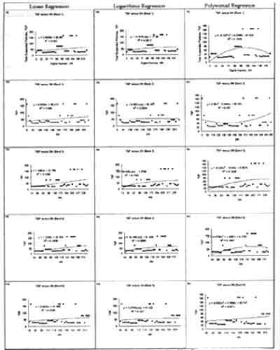
Figure 2: Linear, Logarithmic and Polynomial Regression plot for Band 1, 2, 3, 4 and 5
.../continue
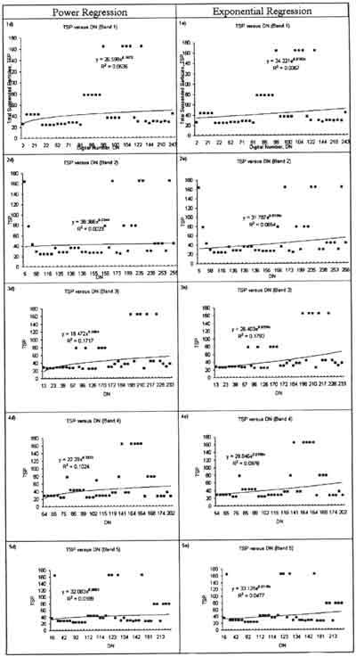
Figure 2(Continued): Power and Exponential Regression plot for Band 1, 2, 3, 4 and 5
| Channel | Coefficient of Determination, R2 | ||||
| Linear Regression y=mx+c |
Logarithmic Regression y=aLn(x)+c |
Polynomial Regression y=ax2+bx+c |
Power Regression y=axb |
Exponential Regression y= aebx | |
| 1 | 0.013 | 0.0613 | 0.1578 | 0.0536 | 0.0357 |
| 2 | 0.046 | 0.0004 | 0.091 | 0.023 | 0.0654 |
| 3 | 0.1486 | 0.1325 | 0.1629 | 0.1717 | 0.1793 |
| 4 | 0.1008 | 0.0999 | 0.1457 | 0.1024 | 0.0978 |
| 5 | 0.0209 | 0.0071 | 0.0212 | 0.0189 | 0.0477 |
The best TSP-DN relationship is shown by exponential regression model of y = 26.4 e0.0229 x with band 3 as input (R2 = 0.1793).
The simplified DN-TSP relationship analysis indicated two preliminary findings : (i) Weak relationship by the best R2 score using IR band 3 of NOAA AVHRR data (there is great tendency of saturation in satellite data that deemed relationship); (ii) TSP are more detectable in IR band (band 3), where of all the tested models, (he highest R2 score is shown each time band 3 is used (see table 2).
Summary
The TSP-DN relationship using NOAA-12 AVHRR data has been examined. Early result of this the study is encouraging, despite weak relationship shown by exponential model of y= aebx, where a, b are constants which varies with the band input. This early results also suggested that the cloud as one of the phenomenon that has hinder good TSP-DN being analyzed. In future the cloud influence will be priorily minimized, apart from analyzing individual relationship of each haze solid particulates matter, gases such as CO2, CO, CH4, etc.) to the corresponding satellite's records.
References
- Goody, R. M. & Walker, J. C. G. (1972) Atmospheres. Eaglewood Cliffs, New Jersey : Prentice-Hall.
- Malaysian Meteorological Service (1995). Report on Air Quality in Malaysia as Monitored by the Malaysian Meteorological Service. Kuala Lumpur : Malaysian Meteorological Service.
- Morris, W (Ed). (1975). The Heritage Illustrated Dictionary of English Language of The English Language. New York: American Heritage Publishing Co.
- Neiburger, M. Edinger, J. G. and Bonner, W. D. (1973). Understanding Our Atmospheric Environment. San Francisco : W. H. Freeman and Company.
- Malaysian Meteorological Service (1995). Annual Summary of Air Pollution Observations. Kuala Lumpur : Malaysian Meteorological Service.