| GISdevelopment.net ---> AARS ---> ACRS 1997 ---> Poster Session 2 |
Retrieval Of Ocean Winds Form
Ers-1/2 Scatterometer And Sar Data Using Natural Network.
K.S.Chem. J.T.Wang * and
A.J.Chem.
Center for space and Remote sensing research *Department of Atmospheric University National Central University Chung-Li, Taiwan
E-mail:dkschen@csrsr.ncu.edu.tw
Abstract Center for space and Remote sensing research *Department of Atmospheric University National Central University Chung-Li, Taiwan
E-mail:dkschen@csrsr.ncu.edu.tw
This paper presents the retrieval of the ocean winds observed from C-band microwaver scatterometer onabord ERS-1 satellite platform I April 1994. the study area was located at west Pacific water area (~ 17n , 124E~25N, 135E). a neural network is adopted to implement the inversion of a geophysical model function which relaters the scatter meter measurements of normalized radar cross section to surface wind speed and direction. To illustrate the functionality of the neural network, a set to wind fields were generated by means of Monte Carlo simulations. At each sample point, the 3ind speed and direction are obtained. Then, a geophysical model function proposed by ESA ( European Space Agency ) was used to produce the simulated normalized radar cross section at three pointing antennae of scatterometer according to the ERS -1 configuration. As a result neural network was constructed as having four imputes nodes accepting three NRSCs and an incident angle at nid-beam antenna, and two output nodes representing the inverted ( and desired ) wind speed and direction. Network training was accomplished by the input output pairs which are randomly selected from the database of simulated wind fields. The effectiveness of the neural network as an inverse transfer function was validated. Applying this well trained neural network to ERS-1 data was presented. Comparisons with traditional optimization method concludes that satisfactory results were able to obtain by the proposed neural network approach. Wh4en makes use of spatial information, improvement of the retrieval accuracy can be obtained. The use of SAR to derive ocean winds is driven by the demands of fine spatial resolution such as in the coast regions. A pair of SAR image data were acquired within the study area of scatterometer with very closely in time. Atmospheric boundary layer rolls ere observable on the image, thus the wind direction was able to determine. The CMOD-4 model was then applied to estimate the wind speed, following a radiometric calibration. No buoy data was available to quantitatively conclude our results. Nevertheless, reasonable agreements were obtained when comported to scatterometer.
Introduction
Scatterometeris microwave radar with capability of relating measured normalized radar cross section to wind speed and direction over the ocean surface. The principles of the scatterometer measuring the wind lies in the fact that the microwave radar echo from ocean surface are dependent on amplitude and density of the waves. These waves are related to wind. In mocrowave region, the Bragg wavelength is in the water wave capillary-gravity waves which are generated by wind [ Moore and Fung, 1979]. The strength of the radar echo also determined by the radar frequency, po9larization and incident angle, as described by radar equation. Hence, scatterometer provides an indirect means of wind field measurements. How-ever , the interaction of the radar signal and owned-roughed sea surface are complicated. For example, the mechanism of the generation of waves by the wind is poorly understood. The relation between the wind at 10 m above the surface and momentum flux into the ocean is dependent on the surface wave structure, the layer strification , and the magnitude of the wind. In addition, recent experiential observations reported that the NRSC may change significantly across a sea surface temperature front . The success and value of scatterometer, therefore, requires a good relationship between the scatterometer signal na surface wind. Practically speaking, there are two basic problems that need to solved: a transfer function that relates the NRCS to wind field, and a method that inverts wind field form NRCS. Mathematically,
V= G(s0 , q, f,p) (2)
Where s0 is NRCS measured by scatterometer, V is surface wind vector ( speed and direction ); ? is incident angle, f is radar frequency, and P is polarization. Note the radar system parameters are know but may subject to nose contanimation.
In the above, G is known as geophysical model function and g is inverse transfer function which is usually a multivalued function. Hence, several measurements of s0 form different azimuth angle must be used to estimate the wind vector . conventional approach to wind estimate involves formulating a cost function from the scatterometer measurements and then minizing it to obtain estimates of wind field. Local minima are usually appear due to the nature of geophysical model function . this leads to the some called aliasing or ambiguity. Since dealiasing or ambiguity removal relies on the information not contained in s0 measurements, it is not pursed here. In this paper, we are primarily concern with the inverse transfer function g. Because it is nonlinear5 and the exact character of the nonlinear behavior may not be known a priori. Neural network offers a highly flexible, yet accurate, alternative to implement the transfer function. In the next section, the scatterometer models are first mentioned to facilitate the sections that follow. Section 3 presents the neural network approach to implementing the inverse transfer function, in particular, a dynamic learning neural network (DLNN) trained by a Lalman filtering technique is applied. The input-output structure of the network and learning algorithm are given. The validation and verification the network are accomplished through numerical simulation.
Scattermoter Models
A series of version of wind scaterometer model for C-band scatterometer onabord ESA ERS-1 satellite have been proposed based on measured data in a global scale. The system parameters of ERS-1 scatterometer was also attached. C-MOD4 is a most updated GMF and is of the form
where j is the relative radar look-wind angle in degree, i.e that his angle is zero when the wind is bellowing towards the radar ; V the wind speed in m/s and ? is radar incident angle in degree. Coefficients b0, b1, and b2 are empirically determined and are given in [Attema, 1991].
Neural Network as inverse Transfer Function
The objective of wind retrieval form scattterometer measurements is to find an inverse function g such that the desired parameters can be obtained form measured data that are available within a sufficient prescision and accuracy. In the design phase of scatterometer, it is desirable that measured data be strongly dependent on the change of wind. The wind fields should be sensible, observable and measurable with the limits of scatterometer specification. Even under these conditions, as usually is, some obstacles were posed however. First, f is intrinsically nonlinear and analytical forms are usually not available. Moreover, the localization properties of the wind fields should be taken into account when searching the optimum solution of f, which should be extremely difficult, if not impossible. Such nonlinear transfer function can be easily modeled use a neural network technique. The capability of generalization and specialization makes it extremely attractive for broad class of remoter sensing problems [ Tzeng, et al. 1994]. In this paper, we apply a modified multiplayer perception structure and training by a Kakman filtering technique called dynamic learning neural network (DLNN).
To exclude the influence of the measurements noise, a set of wind field patterns were first generated using Monte Carlo method [Bartolini et al., 1993]. This can be viewed s noise-free scaterometer measurements obtained with full knowledge of surface truth { wind vector at a given location or pixel ). Thus the retrieval performance of neural network can be evaluated. After sets of wind vectors were generated, the corresponding normalized radar backscattering coefficient s0 values were calculated using a geophysical mode4l function CMOD -4 proposed by ESA, as in (3). At each sample point, three values of s0 which simulate the aft beam, the mid beam, of the ERS-1 scaterometer returns were calculated. The neural network was constructed to have four input nodes, accommodating three s0 values and an incident angle of mid- beam and two output nodes representing the inverted and desired wind speed and wind direction. The input-output relationship was established by CMOD-4. thus no a prori information about the inputs is needed. As input scheme, tow choices are possible: pixel, based and area-based. In pixel -based scheme, the wind speed and direction at each pixel of interest was fully determined by the three s0 alone, while in area-based scheme, they were estimated by including the s0 of all neighboring pixels within a window. The window size, after trial and error, was set by 3 x3. thus, in area-based scheme, a total of 27 s0 measurements were used to determine the wind vector at the point of interest. All points on the boundary, however, can only used pixel-based scheme because of insufficient data within the window. A pool of calculated s0 was randomly divided into two groups : one for training, the wind vectors ( V, j ) can be reconstructed in a straight forward manner. Due to space limitation, only final results are given in fig.1 where we show the truth and inverted values of wind speed and inverted values of wind speed and direction. Very high correlation can be obtained for ERS scatterometer parameter range. Te confidence of DLNN as inverse function is then established .
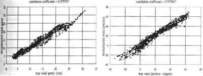
Figure 1: Correlation of wind speed and direction between truth and estimated values
Results and discussion
Due to the absence of ground truth, we compare out results with the wind field reported by ECWMF. The way we compare is to feed ot reconstructed wind vectors into CMOD4 to recover the NRCS which were then checked with the NRCS form scatterometer measurement .
where û, f are reconstructed wind speed and direction, respectively, from DLNN or ECM WF. Each NRCSs from three antenna beam, i.e. fore-, mid-, aft-beam, an the averaged NRCSs were computed. The validation of the CMOD4 however is beyond the scope of this paper. Now, we proceed to recover three backscatter coefficient of three antennas with reconstructed wind field from DLNN and ECMW, followed by calculating the difference between these two sets of backscatter coefficients and measured backscatter coefficients and measured backscatter coefficients. Table 1 list error comparison between DKNN and ECMWF. It is clearly seen that DKNN outperforms ECMWF for all cases. Fig. 2 displays reconstructed wind pattern by DLNN and ECMWF.
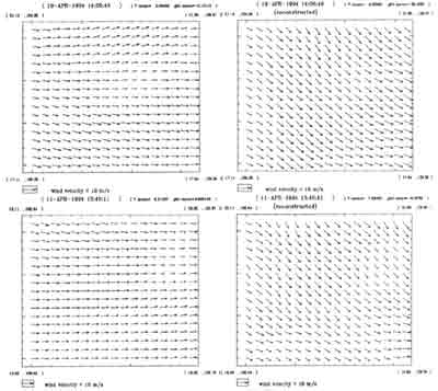
Figure 2: Reconstructed wind field pattern
| Test site | e(ECMWF) | e (DLNN) | ||||||
| f-beam | m-beam | a-beam | Mean | f-beam | m-beam | a-beam | Mean | |
| F14292-38 | 0.00845 | 0.02858 | 0.00850 | 0.01517 | 0.01405 | 0.02326 | 0.00337 | 0.01356 |
| F14292-39 | 0.01201 | 0.00990 | 0.00256 | 0.00816 | 0.00860 | 0.02303 | 0.00245 | 0.01136 |
| F14429-04 | 0.00790 | 0.02886 | 0.00278 | 0.01318 | 0.00326 | 0.01742 | 0.00739 | 0.00936 |
| F14314-05 | 0.01143 | 0.033725 | 0.00255 | 0.01708 | 0.00351 | 0.02153 | 0.00862 | 0.001122 |
| e = s0 ECMF- s0 meansurements | e = s0 DLNN - s0 meansurement | |||||||
Conclusions
The wind reconstructions of C-band scarreometer onboard ERS-1 satellite using neural network was presented. The network structure, training scheme, and input-output configuration was also given. The mapping from antenna measurement to wind field was provided by the CMOD4. four data sets form ERS-1 pass over west pacific were selected for testing. Due to the lack of ground truth data during the satellite pass , retrieval results were evaluated from the recovery performance. The recovered NRCS was compared to the satellite measurements at three antennae. The neural network method gives smaller error for all cases than ECMWF results. Excellent mapping between inputs and outputs can be pr9vided by the neural network. Moreover, the spatial context of the wind field can be easily incorporated into the network inputs. The training time is increase of retrieval accuracy.
References
- Attema E.P.W., the Active Microwave Instrument on -board the ERS-1 satellite, Proceedings of the IEEE, Vol. 79, pp. 791-799, 1991.
- Bartoloni A., C.Damelio, and F.Zirilli, Wind reconstruction from Ku-band of C- band scatterometer data, Journal of Geophysical Research, Vol. 91, pp. 5153-5158, 1986.
- Johnson, J.W., L.A. Willams, Jr., E.M.Bracalente, F.B.Beck , and W.L.Grantham, Seasat-A satellite scatterometer instrument evaluation, IEEE Journal of Oceanic Eng., vol. OE-5, pp.138-144, 1980.
- Liu Y. and W.J.Pierson jr., Comparisons of scaterometer models for the AMI on ERS-1; the possibility of systematic azimuth angle biases of wind speed and direction, IEEE Transaction of Geosciences and Remote sensing, Vol. 32, pp. 626-635, 1993.
- Long A.E., Towards a C-band radar echo model fro the ERS -1 scatterometer," Proceed - ing of the 3 rd International Colloquium on Spectral Signatures of Objects in Remote sensing, ESA SP-247, ESTEC, Noordwijk, The Netherlands, 1986.
- Moore, R.k.and A.K fung, Radar determinations of wind at sea, Proceedings of IEEE vol. 67., pp. 1504-1521, 1979.
- Tzeng Y.C., K.S.Chen, W.L.Kao, and A.K.Fung, ' A dynamic learing neural network for remote sensing applications," IEEE Transaction on Geosciences and Remote sensing. Vol.32, pp. 1096-1102, 1994.