| GISdevelopment.net ---> AARS ---> ACRS 1997 ---> Poster Session 2 |
A Comparison of Bilinear
Interpolation, Cubic Convolution, and Brownian Interpolation with Least
Squares Matching
Jin-Tsong Hwang and
Tian-Yuan Shih
Department of Civil Engineering
National Chiao-Tung University
Hsin-Chu, Taiwan,R.O.C.
Abstract Department of Civil Engineering
National Chiao-Tung University
Hsin-Chu, Taiwan,R.O.C.
This study compares two fractal interpolation schemes based on fractional Brownian motion (fBm) with two convectional interpolation schemes: bilinear interpolation and cubic convolution. Numerical experiments are performed with a pair of digitized stereo photographs. The original image is reduced to a lower spatial resolution for interpolation. Both the geometric index based on the positioning accuracy of the image matching and the statistic indices such as the root mean square error, average error, maximum deviation, and correlation coefficient derived by comparing interpolated and the reference images indicate that the convectional interpolation schemes are better than the Brownian schemes.
Introduction
This paper examines four interpolation techniques: bilinear interpolation, cubic convolution, weighted Brownian interpolation (Polidori and Chorowicz, 1993), and the modified weighted Brownian interpolation derived in this study. The global statistic and geometric accuracy indices of the interpolated images generated by the four interpolation techniques are computed. The statistical indices include root mean square error (RMSE), average error Bias), correlation coefficient (), and maximum deviation, while the geometric index is the positioning accuracy derived from image matching. Two sampling schemes are also applies to reduce the test image into a lower spatial resolution. The first is decimation which takes the Nth pixel every N pixel. The other is averaging which takes the average of (N+1) x (N+1) window every N pixel. Numerical experiments are also performed with the SUBURB dataset provided by ISPRS Working Group III/3. This dataset includes a pair of digitized stereo photographs, as well as the DTM generated from this pair.
The Interpolation Schemes
Weighted Brownian Interpolation (polidori and chorowizc, 1993)
According to fBm (Mandelbort, 1983), the expected value of the difference in grayscale value over the distance dx is proportional to (dx)H where H is a constant and lies in the range 0<H<1, with a Gaussian distribution (Yokoya et al., 1989; Polidori and Chorowizc, 1993). The relationship between parameter H and fractal dimension D is in Equation (1).
Parameter H can be determined by fitting a straight line with Equation (2):
Where both H and K are constant. Equation (2) indicates that a plot of (E[|Z(X+dx)-Z(X)|]) as a function of dx on a log-log plot lies on a straight line and its slope is H (Yokaya et al., 1989).
Let s2 be the variance of grayscale differences over a distance dx that equals one pixel in the input image. If the straight line are extended toward a shorter distance, the variance s21/2 over a distance dx equal to ½ pixel could be obtained with Equation (3):
Further, the variance s2b obtained over ½ pixel by a bilinear interpolation is:
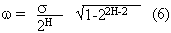
The weighted Brownian interpolation proposed by Polidori and Chorowicz (1993) adds a random term to the bilinear interpolation. The variance of the subsequent model is the difference between s2b and s21/2, as shown in equation (5) (Polidori and Chorowicz, 1993; Saupe, 198):
For random addition, three parameters, w, G, and R, are expressed in Equation (7):
Where Zb(i,j) is the result of bilinear interpolation, G is the Gaussian random variable with a zero mean and unit standard deviation, and R is the correlation coefficient between dx and (E[|Z(X+dx)-Z(X)|])) in the log-log coordinate system. Also, R equals one when the log-log plot yields a straight line. The more the image deviates from the Brownian model implies a smaller R (polidori and Chorowicz, 1993). Because the significance of fractal phenomenon differs from area to area, the purpose of using R is to model the variation of "fractalness". Term w, as described in Equation (6), is formulated with s and H. The two parameters and R are called " fractal factors" in this paper. The image is divided into M*M blocks and each block has N*N pixels. Fractal factors are computed for each block. Then the image is interpolated on the basis of equation (7) block by block with the corresponding s, H, and R. Considering both the computing effect and local representation using the window is inappropriate. Polidori and Chorowicz (1993) recommended using the window size of 13*13 pixel.
Modified Weighted Brownian Interpolation
The term G in Equation (7) is extended to include a thresholding procedure, and is then denoted as GT, as shown in Equation (8):
The random numbers generated are accepted only if they are within the thresholding interval. This thresholding procedure is designed to provide another mechanism to effectively control the added fractal-enhancement components.
Data for Numerical Experiment
The SUBURB dataset released by the Working Group III/3 of International Society for Photogrammetry and Remote Sensing (ISPRS), is used in this study. This dataset consists of a digitized b/w stereopair and a DTM. The scene of this stereopair is primarily a group of single-family, one- to three-floor suburban homes surrounded by gardens and trees. The DTM was derived with MATCH-T (INPHO-GmbH, Stuttgart, Germany), from this stereopair.
The right and left images are named SUBURB_R.PGM and SUBURB_L.PGM respectively. The images are in epipolar geometry, and both sizes are 1000*1000 pixels The file name of the DTM is SUBURB.DTM, containing three-dimensional coordinates in the terrain system. The planimetric spatial resolution of this DTM is one meter.
Image Data Preprocessing
The Fractal Factors and Image Reduction
The fractal property is examined with Equation (2) in all directions and shown in Table1.
| Sampling type vs. reduction ratio | Range of pair distance | Decimation sampling | Averaging sampling | ||
| H | R2 | H | R2 | ||
| Original | (1-23) | 0.5544 | 0.9922 | - | - |
| Reduction ratio 1/2 | (1-12) | 0.5108 | 0.9944 | 0.5689 | 0.9915 |
| Reduction ratio 1/4 | (1-6) | 0.4714 | 0.9964 | 0.5633 | 0.9938 |
| Reduction ratio 1/8 | (1-4) | 0.4231 | 0.9982 | 0.5537 | 0.9965 |
| Reduction ratio 1/16 | (1-11) | 0.0618 | 0.9614 | 0.0881 | 0.9729 |
The stereo-pair's left image is selected for reduction. The reduction ratios are chosen to be 1/2, 1/4, and 1/8. Both the decimation and averaging scheme are adopted. The six reduced images, three for each sampling scheme, are then interpolated back to the original image size with the afore-mentioned four interpolation schemes.
Target Points of Least Matching
The data points in the DTM dataset SUBURB.DTM are transformed into an epipolar coordinate system and then to a row and column system. After transformation, each point in SUBURB.DTM corresponds to a stereo-point pair located on the left and right images. Let the point on the left image be a target point. The point on the right image would then be the conjugate point for correct matching. In this study, 849 points well-distributed around the center of the left original image are selected as the target points. Results obtained from image matching are transformed to ground coordinates and then compared with the ground truth in the SUBURB.DTM file .The RMSE of the coordinates between the results from image matching and ground truth function as the index of positioning accuracy.
Results and Analysis
These groups of indices are used for evaluation: statistic, fractal, and positional.
The statistic indices include RMSE, Bias, correlation coefficient (r), and maximum deviation. Those indices are computed from the grayscale differences between the interpolated and the original. Based on the considerations of local representation, fractal factors were estimated over a square window. Different window sizes are used for images of different reduction ratios. In this study, the sizes were 50*50, 25*25, and 12*12 for reduction ratios ½ ,1/4, and 1/8, respectively.
Roy et al. (1987) recommended computing the fractal dimension from the Richardson plot with pair-distance intervals up to ¼ of the maximum distance on the image. According to Table 1, the fractal property of the reduction ratio ½ lies within the distance from one to twelve pixels. Although 4 times 12 equals 48, the size of the square window was set at 50*50 for the computation. Based on the same strategy, the window sizes 25*25 and 12*12 were used for the reduced images with reduction ratios ¼ and 1/8 respectively. Comparing with the 13*13 window used for the ¼ reduction ratio in Polridori and Chorowicz (1993), reveals that the fractal dimension computed from the current research is more significant.
After the square window was defined, each reduced image was divided into 64 square blocks, i.e., each block is 50*50pioxels for the 401*401 image (reduction ratio: 1/2), 25*25 for the 201*201 image (reduction ratio: 1/4), and 12*12 for 101*101 image (reduction ration: 1/8). Therefore, for each reduced image, there were 64 sets of fractal factors.
The term G in the weighted Brownian interpolation method proposed by Polidori and Chorowicz (1993) is a Gaussian random variable with zero mean and unit variance. The modified version introduces a threshold to G to effectively control the fractal enhancement. The threshold was selected as 0.3 based on the success rate of image matching. Therefore, the random values introduced in the fractal interpolation scheme were within -0.3 and 0.3.
| Interpolation methods | Type of sampling | RMSE (pixel) | Bias (pixel) | s | Max. |
| Bilinear | Decimation | 10.826 | 0.796 | 0.975 | 130 |
| Averaging | 12.104 | 1.242 | 0.969 | 130 | |
| Cubic convolution | Decimation | 9.630 | 0.021 | 0.979 | 133 |
| Averaging | 10.037 | 0.435 | 0.978 | 133 | |
| Fractal interpolation (no threshold) | Decimation | 19.570 | 1.016 | 0.920 | 151 |
| Averaging | 16.115 | 1.482 | 0.942 | 148 | |
| Fractal interpolation (threshold 0.3) | Decimation | 11.175 | 1.034 | 0.973 | 132 |
| Averaging | 12.266 | 1.486 | 0.969 | 131 |
From the statistic indices, several observations can be made.
- When the enlargement ratio is increasing, the statistic indices indicate that the quality of interpolation is deteriorating. This could be well accounted for by the image's lower information content with a larger reduction ration.
- Cubic convolution performed the best while weighted Brownian interpolation was the worst. The modified version displayed an improvement over the original scheme. The reason for this poor showing could be caused by the manner in which the fractal factors were computed. The random term of Equation (7) was obtained by multiplying the Gaussian random numbers and fractal factors. The weighted Brownian interpolation method interpolates images block by block, and each block has its own fractal factors so that the interpolated image resembles a mosaic pattern.
- Results obtained from images reduced with the averaging scheme were worse than those from images reduced with decimation scheme. This phenomenon may be related to the low-pass effect of the averaging process.
The H values for each interpolated images are computed with the variogram method. The result shows that H value of the averaging scheme produced image was closer to the one of the original than the one produced by the decimation scheme. This finding is quite interesting, indicating that from the perspective of fractal preservation, averaging process is better than the decimation process.
The weighted Brownian interpolation yielded the lowest H value among all four interpolation schemes. That is, the image enlargened with weighted Brownian interpolation without thresholding has the highest fractal dimension.
Positioning Accuracy with Least squares Matching
The least squares matching method was adopted in this paper to evaluate the positioning accuracy of these four interpolation methods. To attain a sub-pixel order, the iteration is terminated when one of the following conditions is fulfilled: the translation increment is less than 0.01 pixel or the iteration number is larger than 20. Tables 3 summarize the results of this comparison for x4 enlargement.
| Positioning accuracy vs. Interpolation methods | Type of sampling | Success rate (%) | X-RMSE (m) | Y-RMSE (m) | Z-RMSE (m) |
| Bilinear | Decimation Averaging |
75.4 | 0.1270 | 0.2757 | 0.6263 |
| 76.8 | 0.1389 | 0.2999 | 0.6741 | ||
| Cubic convolution | Decimation Averaging |
74.1 | 0.1238 | 0.2610 | 0.5887 |
| 77.6 | 0.1260 | 0.2702 | 0.6046 | ||
| Fractal interpolation (no threshold) | Decimation Averaging |
2.0 | 0.1385 | 0.3304 | 0.7317 |
| 33.2 | 0.1478 | 0.3182 | 0.7493 | ||
| Fractal interpolation (threshold 0.3) | Decimation Averaging |
63.6 | 0.1296 | 0.2680 | 0.6331 |
| 68.9 | 0.1329 | 0.3006 | 0.6559 |
According to the comparisons for all enlargements, the RMSEs of both fractal approaches are larger than those obtained with convectional interpolation schemes. Even the success rates are also lower. The modified version shows some improvement, but is placed between the convectional schemes and the fractal approach. As for sampling, the averaging scheme yielded a higher success rate than the decimation scheme. However, in terms of positioning accuracy from matching, no significant difference arises.
Concluding Remarks
Contrary to what was expected in the beginning of this study, the weighted Brownian interpolation schemes were not found to be better than convectional resampling algorithms, bilinear and cubic convolution. Instead, the result is inferior to those from conventional approaches in terms of both statistic indices, such as correlation coefficients, RMSE, and the geometric index from the positioning accuracy of image matching. In terms of fractal preservation, evaluation of fractal based approaches is reasonably well, but with exceptions.
Why the fractal based schemes provide inferior interpolation results than the convectional schemes? A possible explanation is that the fractal interpolation under study, introduces the fractal components using a random number generated as the core. Even if a true fractal process can be generated in this manner, it may not be the same iterated function system as the one governing the image to be interpolated.
References
- Mandelbrot, B.B., 1983. The Fractal Geometry of Nature. W.H. Freeman and Company, New York, 468pages.
- Polidori, L., and J. Chorowicz, 1993. Comparison of Bilinear and Brownian Interpolation for Digital Elevation Models. ISPRS Journal of Photogrammetry and Remote Sensing, 48(2): 18-23.
- Yokoya, N., K. Yamamoto, and N. Funakubo, 1989. Fractal-Based Analysis and Interpolation of 3D Natural Surface Shapes and Their Application to Terrain Modelling. Computer Vision, Graphics, and Image Processing, 46: 284-302.