| GISdevelopment.net ---> AARS ---> ACRS 1997 ---> Poster Session 2 |
Marine Gravity Recovery for
the Malaysia Region from TOPEX, ERS-1 and Geosat Satellites Radar
Altimeter Data
Shahrum Ses, Majid Kadir
and Hassan Hashim
Faculty of Geoinformation Science and Engineering
University Technology Malaysia
Locked Bag 791
80990 Johor Bahru, Malaysia
E-mail:sharum@fksg.utm.my
Abstract Faculty of Geoinformation Science and Engineering
University Technology Malaysia
Locked Bag 791
80990 Johor Bahru, Malaysia
E-mail:sharum@fksg.utm.my
Over the last 20 years, considerable developments in the measurement of sea surface heights using a satellite radar altimeter have been observed. The measurement precision has improved from 300cm to 2cm the and the resolution has been reduced from 70km to less than 20km on the ground. The dense satellite altimeter data gives an insight into the detail recovery of marine gravity field which can be used for geological exploration of the sea floor.
The combined Topex, ERS-1 and Geosat altimeter data have been used for the determination of the sea surface (MSS) and marine gravity field in the Malaysian region (j=00 to 100, l=960E to 1200E). A substantial amount of the combined altimeter records have been used in the elevation. The gravity field was derived from the height anomalies using Fast Fourier Transfer (FFT) technique. The free air gravity anomalies were obtained on a regular grid of 3'45" * 3'45" corresponding to 7km spacing at the equator. The precision of the satellite altimeter derived gravity anomaly values over the open marine area of the Malaysian region is expected to the better than 2mGal. The quality of anomaly recovery in the semi-enclosed seas around the region was also verified by comparison with the available shipboard measurements.
Overview on the Altimetry Missions
Radar altimeter measurements of the sea surface height gave marine geodesists and geophysicists an insight into the detail recovery of gravity field over all the ocean and basins. Experience with GEOS-3 and Seasat in the 1970s had demonstrated the enormous potential of altimetry, but neither mission provided such complete long-term global coverage. From March 1985 until January 1990, the U.S. Navy satellite Geosat generated a new data set with unprecedented spatial and temporal coverage of the global oceans (Dougals and Cheney, 1990). Geosat paved the way for a series of highly-successful altimeter missions that followed it, i.e. ERS-1 (!((!-96), TOPEX/POSIEDON (1992-), and ERS-2(1995-).
The inclination and the repeat period determine how the altimeter data will be distributed on the earth. Geosat has an inclination of 1080 which means that the satellite's ground tracks are located between -720 and 720 latitude. Since the ERS-1 has an inclination of 980 , the covered area is extended by 100 south and north. The period, at which the satellite completes one revolution also determines the pattern of satellite's ground tracks on the surface of the earth. The repeat period of the satellite orbit governs the spacing of the altimeter tracks on the ocean surface. Longer repeat cycles such as 168-day ERS-1 geodetic phase or the non-repeat (drifting) orbit of the Geosat GM provide the high-density coverage of the altimeter tracks.
The acronym "Geosat" was derived from geodetic satellite, because its primary mission was to obtain a high-resolution description of the marine geoid up to latitudes of 72 degrees. This goal was achieved during the first 18 months, known as the geodetic mission (GM). During this time the ground track had a near-repeat period of about 23 days (330 revolutions in 23.07 days). The drifting orbit resulted in a dense, global network of sea level profiles separated by about 4km at the equator. Because of the military significance of this unique set of observations, the GM data were initially classified but in 1995 were released to NOAA in their entirely for public distribution. At the conclusion of the GM on September 30, 1986, the satellite orbit was changed, and the exact repeat mission (ERM) began on November 8, 1986. This produced sea level profiles along sea track that repeated themselves within 1-2 km at intervals of about 17 days (244 revolution in 17.05 days). The ERM covered 62 complete 17-day cycles before tape recorder failure in October 1989 terminated the global data set.
The global coverage of the European Earth Resource Satellite (ERS-1) altimeter data (up to latitudes of 80 degrees) have been used for the determination of the marine gravity field. The use of the one year 35-day repeat ERS-1 data (from November 10, et alkalinity., 1992; Yi, 1995; Hwang, 1997). The shorter repeat periods of 35 days for ERS-1 do not provide dense track coverage. On April 10, 1994, the ERS-1 satellite went into its first 168-day repeat cycle, the so-called geodetic phase. Very long repeat cycles of 168-day for ERS-1 geodetic mission provide the high-density coverage needed for complete resolution of the gravity field.
Altimetry-derived Sea Surface Heights
The satellite serves as a stable platform from which a radar altimeter can measure the distance to the instantaneous ocean surface. The radar altimeter works by transmitting a short pulse (approximately 3 nanoseconds). By measuring the travel time of the pulse it is possible to obtain data on the shape of the sea surface. A simplified geometry of a radar altimeter can be written as follows:
where hSSH is the sea surface height (SSH) above the reference ellipsoid, h is the satellite altitude above the reference ellipsoid, and r is the distance from the footprint on the sea surface to the satellite.
The altimeter data is usually given as a set of geophysical data records (GDR) that include altimeter measurement information, as well as corrections that should be applied to the data. In mathematical terms the altimetric observation of the sea surface height can be described according to the following expression:
where N is the geoid height, S is the sea surface topography, and e is the error. The error term of equation (2) can be described as follows:
where e0 is the radial orbit error, eT is the ocean tide residuals, eA is additional errors (eg. Wet troposhperic correction), and n is the measurement noise.
The noise of the measurements is in the order of a few centimeter. The largest error component is the radial orbit error, which is split into an errors caused by geopotential errors and errors caused by initial state vectors errors, drag, and solar radiation pressure. The second largest error term is not related to the altimeter measurement itself. The tidal models which has an accuracy of around 10m were applied in order to convert an instantaneous sea surface height into a mean sea surfaces height.
New gridded data sets of mean sea surface (MSS) were produced on 30 45"grid using one-year mean sea surface height (SSH) data of Geosat, ERS-1 and Topex altimeter satellites (Yi, 1995). An inverted barometer correction and improved ocean tide correction (Cartwright and Ray, 1990) were applied to all SSH data used in this study. A gridding method of the least-squares collocation (LSC) based on the covariance function of the second-order Markov process was used. The residual SSH data were gridded after removing the reference geoid undulation implied by the JGM-3 potential coefficient model. The grided MSS values were computed by adding the reference geoid undulations back to the gridded residual SSH values.
Recovery of Gravity Anomalies form Altimeter
There are three well known techniques used for the recovery of free-air gravity anomalies from satellite altimeter. The first involves converting vertical deflections a attained from SSH that is widely used by geophysicists (Haagmans et alkalinity., 1995; Sanwell and Mcadoo, 1998), and the second is by LSC, which was developed by geodesists (Rapp, 1079; Basic and Rapp, 1992). The third approach which has been used in this study involves direct conversion of Geoid undulations to free-air anomalies using Fast Fourier Transform (FFT) technique (Kim, 1996). After reasonable approximations, a direct relation between geoid undulations and gravity anomalies is given as follows (Heiskeanen and Moritz, 1967).
| Dg= - | ¶ ----- ¶R |
(Ng)- | 2 ---- R |
(Ng) (4) |
Where T is the disturbing potential, N is the geoid undulation, g is the normal gravity and R is the radius of the earth. The first term on the right hand side of equation (4) is called the gravity disturbance (dg) that can be directly calculated by the FFT technique using satellite altimeter SSH for N. Following Kim (1996), for T=gN on the x-y plane, dg is the calculated by the inverse Fourier transformation as:
Where TKl(z) is the 2-D Fourier transformation of Txy at the wave numbers k and l. M and N is the data points in the x and y directions x is the coefficient of the Fourier wave number given as:

Since the data (T= gN) are given on the sea surface with geographical coordinate system ( j, g) for the limited area, a planner and map projection approximation are necessary for actual computations.
Regional Marine Gravity Field Determination
The extent of the area that cover the Malaysia Exclusive Economic Zone (EEZ) is bounded by j=00 to 100 and g=960 to 1200. The geographical setting of the related marine area represents the South China Sea in the East and the Malacca Strait in the West. Generally the coastal waters of the South China Sea are quite shallow and gradually deepen toward the open sea. The bottom topography of this marine region is largely represented by the 400km wide Sunda shelf which is almost flat with about 40m to 100m depth. However, some interesting features is observed in the east with the deep sea floor which is known as Sabh Trough area. The depth of the Malacca Strait varies from about 100m in the north to less than 20m in the narrower part of less than 50km wide in the south.
The reference field used in the predictions is the OSU91A field complete to degree and order 360. The predicted gravity anomalies refer to the ellipsoid of the Geodetic Reference System 1980 (a=6378137m, f=1/298.257). The predicted anomalies provide a uniform (3'45" * 3'45") data set for the marine areas of the Malaysian region. The plots of the anomalies over the marine region are shown in Figure 1 in mGals. The computed values of the marine anomalies in the region vary from -20mGal to about 100mGals. Clearly the Variations is closely associated with the sea floor topography of the region.
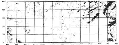
Figure 1: Altimetry derived marine gravity anomaly for the Malaysian region.
Figure 2 shows the gravity variations in the coastal and offshore areas of Terengganu. The gravity anomaly field over this area indicates a rather smooth field with the exception of several pockets of low (-20mGals) anomalies. Also clear from this figure is the smoothing of the field near the land areas since altimeter data are simply not available. Meanwhile the plot of the derived anomaly field over the north-west Sabah offshore area is shown in Figure 3. Two prominent anomaly features can be distinguish from this figure. First, the high anomalies region (40 to 80mGAls) stretching from the upper right to lower left hand corners of the plot that reflect the signatures of the islands in this area, namely, Commodore Reef, Mariveles Reef and Swallow Reef. Second, the low anomalies region (-20 to -40mGals) located to the east of the high anomalies region which can be associated with the bathymetry of the ocean crust of the Sabah Trough area.
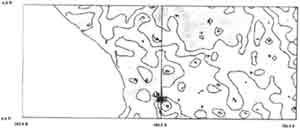
Figure 2: Gravity variations in the coastal and off-shore areas of Terengganu
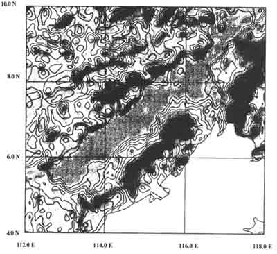
Figure 3: The altimetry derived anomaly field over the north-west Sabah offshore area.
Comparison of Altimetry-derived Marine Gravity Anomalies
Insight on the errors in estimating free-air gravity anomalies from altimetry SSH may be obtained by comparing the values against ship-borne measurements. Altimetry-derived anomaly values were interpolated at 576 shipboard data points disturbed in the northern part of the Malacca Strait. The RMS difference between altimetry-derived anomalies and ship values in this area is 5.42mGals and the mean difference is -0.68mGals (see Table1). Results from cross track comparisons indicated that the ship data contained a reasonably constant error of ~5mGals (Ses, 1997). Assuming that the differences between altimetry and ship data (5.42mGals) were mainly attributed to the error in ship data, the accuracy of the altimetry-derived anomalies in this area is better than +2mGals.
| Statistic of Differences | Northern Malacca Strait (mGals) | South China Sea (mGals) |
| No. of data | 576 | 393 |
| Min | -9.99 | -9.93 |
| Max | 9.85 | 9.98 |
| Mean | -0.68 | 1.04 |
| RMS | 5.42 | 4.52 |
The altimetry-derived anomalies were also interpolated at 393 ship data points in the eastern offshore area of the Peninsular facing the open South China Sea. Better agreements between two data sets were observed over this area with an RMS difference of 4.52mGals (see Table 1). This is possibly due to better than usual shipboard values although this could not be verified due to paucity of cross track ship information over the area.
Conclusion
This study has clearly indicated the ability of the altimeter data to yield a detailed mapping of the gravity field in the ocean areas. The combined Topex, ERS-1 and Geosat altimeter data have been used for the determination of the mean sea surfaces (MSS) and marine gravity field in the Malaysian region ( j=00 to 100N, l=960E to 1200E). The gravity field recovery involves direct conversion of geoid undulations to free-air anomalies using Fast Fourier Transform (FFT) techniques. A substantial amount of the combined altimeter records have been used in the evaluation of free air gravity anomalies on a regular grid of 3'45" * 3'45" corresponding to 7km spacing at the equator. The precision of the satellite altimeter derived gravity anomaly values over the open marine area of the Malaysian region is expected to be better than 2mGal. It has also been shown that the dense altimeter data gives an insight into the detail recovery of marine gravity field, which can be used for geological exploration of the sea floor.
References
- Basic, T. and R.H. Rapp, 1992. Ocean wide prediction of gravity anomalies and sea surface heights using Geos-3, Seasat and Geosat altimeter data and ETOPO5U bathymetric data. Report No. 416, Dept. of Geodetic Science and Surveying, The Ohio State university, Columbus.
- Cartwright, D.E. and R.D.Ray, 1990. Oceanic tides from Geosat altimetry. Journal Geophys. Res., 95, 3069-3090.
- Douglas, B.C. and R.E. Cheney, 1990. Geosat: Beginning a new era in satellite oceanography. Journal Geophys. Res., Vol.95, No.C3, 2833-2836.
- Haagmans, R., development Min, E. and M. van Gelderen, 1995. Fast evaluation of convolution Stokes integral. Bulletin Geodesique,70.
- Heiskanen, W.A. and H. Moritoz, 1967. Physical Geodesy. W.H. Freeman and Condition., San Francisco and London.
- Hwang, C., 1997. Analysis of some systematic errors affecting altimeter-derived sea surface gradient with application to geoid determination over Taiwan. Journal of Geodesy, 71:113-130.
- Kim, J.H., 1996. Improved recovery of gravity anomalies from dense Altimeter data. Report No.437, Dept. of Geodetic Sciences and Surveying, The Ohio State University, Columbus.
- Knudsen, P., Andersen, O.B. and C.C. Tscherning, 1992. Altimeter gravity anomalies in the Norwegian-Greenland Sea-Preliminary results from the ERS-! 35 days repeat mission. Geophys. Res. Lett., Vol. 19, No.17, 1795-1798.
- Rapp, R.H., 1979. Geos-3 data processing for the recovery of geoid undulations and gravity anomalies. Journal Geophys. Res., Vol.84, No.B4, 3784-3792.
- Sanwell, D.T. and D.C. McAdoo, 1988. Marine gravity of the southern ocean and Antartic margin from Geosat. Journal Geophys. Res., Vol.93, No.B9, 10389-10396.
- Sen, S. 1997. The need and prospects for a new height control of Peninsular Malaysia. Ph.D.Thesis, University of South Australia, Adelaide.
- Yi, Y., 1995. determination of gridded mean sea surface from Topex, ERS-1 and Geosat Altimeter data. Report No. 434, Dept. of Geodetic Science and Surveying, The Ohio State University, Columbus.