| GISdevelopment.net ---> AARS ---> ACRS 1997 ---> Poster Session 2 |
Multi-Sensor Radiometric
Correction: A Case Study from Malaysia
Muhamad Radzali Mispan* and
Paul M. Mather
Department of Geography, University of Nottingham
University Park NG7 2RD Nottingham
United Kingdom
*Present address: Senr, Mardi,
P.O. Box 12301, 50774 Kuala Lumpur,
E-mail: radzali@mardi.my
Abstract Department of Geography, University of Nottingham
University Park NG7 2RD Nottingham
United Kingdom
*Present address: Senr, Mardi,
P.O. Box 12301, 50774 Kuala Lumpur,
E-mail: radzali@mardi.my
Remote Sensing offers practical benefits in our understanding about the nature and characteristics of land surface features. However, cloud cover normally impedes the use of optical remotely sensed data in studies of low-latitude regions (tropical areas). Therefore, data from different sensor such as Landsat TM and SPOT HRV are required to ensure as complete a temporal coverage as possible. These however, increase the complexity of the analysis as the SPOT-HRV and Landsat TM sensors have different characteristics and acquire data under different atmospheric, viewing and illumination conditions. In this study, the radiometric correction required to ensure compatibility of data over time and between sensors are described. Calibration to adjust sensor drift was performed followed by atmospheric correction based on combination 6S model and Dark Dense Vegetation (DDV) method. Next, data from different sensors (TM and SPOT HRV) were adjusted for sensor characteristics (band pass) and viewing conditions. The radiometric correction process will not only, correct the image data but also convert them to radiance or reflectance factor for quantitative analysis. The procedure is illustrated using a case study from Malaysia.
Introduction
Ideally, a comparison of several satellite scenes over a period of time, covering the same area, would show changes in the intrinsic properties of land surface features. Such changes in spectral response, however, may also be due to effects related to sensor performance, atmospheric condition at the time of over pass, and viewing and illumination geometry of the sensor. Hence, the use of data from different sensors to provide better temporal coverage results in an increase in the complexity of data analysis as each sensor has different characteristics. Therefore, there is a need to calibrate and correct these data spectrally and spatially and convert to a common scale or datum, so that they are internally (within scene) and externally (between scene) consistent. This paper demonstrates a radiometric correction technique applied to data acquired by two different sensor systems and subsequently makes sensible comparison between images. It places emphasis on establishing a spectral datum for operational, use of this technique.
Material and Methods
Radiometric correction of multi-sensor data involves three steps: sensor calibration, atmospheric correction, and sensor inter-calibration. This study used a combination of 6S radiative transfer code and pseudo-invariant objects. For sensor calibration and atmospheric correction, dark dense vegetation (DDV) was used as a spectral datum. For sensor inter-calibration, DDV and other pseudo-invariant objects available in the image data were used to compensate for the effect of different of different sensor characteristics and view geometry between Landsat-TM and SPOT-HRV sensors.
Resources
The study area is located at the central western coast of Peninsular Malaysia (Latitude 30 25' N and longitude 1010 45' E) about 20km south of Kuala Lumpur. This study used Landsat -5 Thematic Mapper (TM) and SPOT HRV-2 data acquired on the 6 March 1990 and 26 December 1990 respectively (Table 1). The image processing and analysis were carried out using ERDAS-Imagine software at the Department of Geography, University of Nottingham.
Sensor calibration
A linear model relates the digital value (DN) of an image pixel to the intensity of reflected radiant energy (L) (Wm-2 sr-1mm-1). In order to calculate the radiance for a given pixel (i,j) in a spectral band (l), the calibration gain (A) and offset (B) must be known. However, the accuracy of the calibration coefficients of Landsat TM data stored in the tape header are limited by the undocumented performance of the sensor and the ground receiving station (Price, 1087). Thus the calibration gain and offset values must be updated if accurate results are to be achieved. This study uses a method proposed by Olsson (1995) to derive calibration coefficients for Landsat TM data. This method gives a better estimate of the coefficients (Mispan, 1997). However for SPOT-2 HRV data, the study uses the absolute calibration gain provided in the tape header. Table 1 shows the calibration gain and offset of the Landsat TM images. The relationship can be expressed using equation (1) for Landsat-5 TM and equation (2) for SPOT HRV-2 data:
Lli = DNli | Ai (2)
| Band | Green | Red | NIR | |
| TM-90 | Ai | 1.174 | 0.806 | 0.816 |
| Bi | 6.05 | 3.36 | 3.25 | |
| SPOT2-HRV1 | Ai | 1.067 | 1.177 | 1.289 |
| Bi | 0 | 0 | 0 |
Atmospheric correction
The basic philosophy of atmospheric correction is to obtain information about the atmospheric optical characteristics and to apply this information in a correction scheme (Kaufman, 1989). It is a process of surface reflectance retrieval, rs, from the corresponding reflectance at the top of atmosphere, or simply apparent reflectance, r*. The relationship between the radiance, L, of spectral band li , and the apparent reflectance can be expressed using equation (3):
| r* (li) = | L(li) ------------ Ex.d.Cos(q) |
(3) |
Where Es is the exo-atmospheric solar irradiance at the top of the atmosphere (Wm-2 sr-1mm-1), d is the distance multiplicative factor (unit less) and q is the solar zenith angle (degree). Subsequently, the relationship between apparent reflectance and surface in the present of atmospheric constituents can be expressed as follows:
Where ra is atmospheric reflectance, DÆ is the relative azimuth between sun and satellite direction, S is the atmospheric spherical albedo, T(li.qs) and T(li.qv) are the scattering transmittance in the solar and sensor direction respectively and T g(li.qs.qv) is the gaseous absorbing transmittance. A detailed description of this relationship can be found in Tanre et al. (1990).
This study employs a combination of the method proposed by Moran et al. (1992) and Kaufman and Sendra (1998), i.e. using the 6S radiative transfer code and tropical forest cover as the controlled dark dense vegetation (DDV) to derive the aerosol optical thickness and to correct for atmospheric effects on remotely sensed images. The reflectance of tropical forest is in the range of 1-2% in the blue (0.4-0.5 mm) and red (0.6-0.7 mm) region, and 2-3% in the green (0.5-0.6 mm) region (Kaufman, 1989). The 6S radiative transfer model was first used to determine the atmospheric optical characteristics at the time of each satellite overpass. The tropical atmospheric model and maritime aerosol model were used to represent the atmospheric condition at the time of satellite overpass. These models are representative of atmospheric conditions in the Malaysia environment (Mispan, 1996). Given the atmospheric optical characteristics of each spectral band, the inverse of the 6S model was used to retrieve the surface reflectance of the DDV. The inversion equations are as follows:
| A1 = | 1 -------------------- Tg(qs, qv)T(qs)( qv) |
(5) |
| B1= - | ra(qs, qv,Æ) ---------------- T(qs,)( qv) |
(6) |
| Y = A1 r*+ B1 | (7) | |
| rs= | y ------------- (1+SY) |
(8) |
where A1 is the multiplicative coefficient, B1 is the additive coefficients and Y is the atmospheric correction factor.
Sensor inter-calibration
The different between the central wavelengths and viewing angle of SPOT-HRV and Landsat-5 TM spectral bands are large enough to introduce a supplementary variability in the spectral response of a given target and need to be adjusted. This study adopts a method proposed by Muller (1993) to reduce these effects. Invariant objects available on these two data sets were used to derived correction coefficients. Sample points from each pseudo-invariant object were extracted from atmospherically corrected Landsat and SPOT images, and for each sample the mean and standard deviation were computed. The relationship between off-nadir of SPOT-HVR and Landsat-TM data is as follows:
Where
A0=x0-x.s0/s (11)
X0 and s0 are the mean values and the standard deviation of pseudo-invariant objects in the reference image (Landsat TM data) and x and s are the mean value and standard deviation of the pseudo-invariant objects in the image to be corrected (SPOT_HRV data).
Results and discussion
In the absence of in-situ ground measurement simultaneously with the satellite overpass, radiometric corrections to compensate for sensor drift and atmospheric effects can be carried out using scene information and meteorological data. The combination of the inverse 6S model and the dark dense vegetation (DDV) technique can be used to estimate aerosol loading in areas where ground measurements are not available for atmospheric correction. This method is more appropriate in Malaysia, as DDV can easily be extracted from areas under forest cover, Table 2 presents a summary of radiometric corrections carried in this study for both SPOT and Landsat data.
| SPOT-HRV 1 | Landsat - TM | |||||
| Band | 1 | 2 | 3 | 2 | 3 | 4 |
| DDV | 47 | 30 | 101 | 28 | 28 | 77 |
| Radiance | 44.466 | 25.855 | 78.669 | 39.427 | 26.653 | 66.175 |
| Apparent Reflectance | 0.099 | 0.067 | 0.312 | 0.086 | 0.068 | 0.251 |
| Surface Reflectance | 0.054 | 0.035 | 0.348 | 0.043 | 0.037 | 0.275 |
| Sensor inter-calibration | 0.044 | 0.036 | 0.278 | |||
In order to illustrate the difference quantitatively, reflectance value of selected cover types found the study area are extracted from each spectral band of the data sets. Figure 1 compares the reflectance value in the homologous channels of SPOT HRV and Landsat TM data. The X-axis of each graph represents the cover type shown in table 3. The left column presents the apparent reflectance and the right column presents the surface reflectance of the image data. In general, the radiometric methods proposed in this study show the ability to bring data from both sensor systems to a common scale. In the green channel (a and b), the apparent reflectance of the DDV (2) between SPOT and Landsat is about 6-8%. After the correction, the values reduce to about 2-3%. A similar proportion of pixel value reduction is also observed in other cover types, except in land cover 9 and 10 where the difference between surface reflectance increases to about 5%. These land covers (9 and 10) are areas where distinct change occurs. The same situation also can be observed in the red channels (c and d). Although the difference between SPOT and Landsat data is minimal in relative unchanged cover types, the increase in spectral values of about 10% are observed in land cover types 9 and 10.
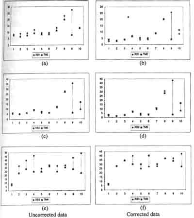
Figure 1: Comparison of spectral reflectance of various covers types derived from raw and corrected SPOT-2 HRV1 and Landsat-5 TM data (see table 3 for list of covers types).
Unlike the visible channels, the near-infrared channel exhibits slight difference in spectral response patterns among the cover types. In the uncorrected data, the reference DDV (cover type 2) shows a substantial difference between XS3 and TM4 (10%). However, the value can be reduced to a common value after radiometric correction is carried out. By bringing the DDV value to a common spectral value, the radiometric effects on others cover types are also reduced accordingly. Based on knowledge of the area, land cover types 3 and 8 also represent relatively stable components between the data acquisition dates. Before corrections are applied, significant differences in reflectance values are observed. However, after correction, the difference is almost negligible. This is in contrast with cover types, which experience change over time such as cover types 4, 5, and 6. The differences in reflectance value for these cover type are enhanced after the correction effort.
| No | Class_Name |
| 1 | Water |
| 2 | Forest |
| 3 | Mature Oil Palm |
| 4 | Young Oil Palm |
| 5 | Mature Rubber |
| 6 | Stressed Rubber |
| 7 | Mixed Horticulture |
| 8 | Bare soil/urban area |
| 9 | Vegetation to Bare |
| 10 | Bare to Vegetation |
Acknowledgements
The authors express their gratitude to the Director General of the Malaysia Agricultural Research and Development Institute (MARDI) for financial report during the study, and to colleagues at the Department of Geography, University of Nottingham, for their support and encouragement. The Malaysia Remote Sensing Center, Kuala Lumpur, kindly supplied the satellite data used in this work.
References
- Kaufman Y.J. 1989, The atmospheric effect on Remote Sensing and its corrections. In Asrar G. (ed.).Theory and applications of optical Remote Sensing . John Wiley & Son. New York, 336-428.
- Kaufman Y.J. and Sendra, C. 1988, Algorithm for automatic atmospheric corrections to visible and near-IR satellite imagery, International Journal of Remote Sensing, 9, 1357-1381.
- Mispan, M.R., 1997, Multi-sensor Remote Sensing data for change detection: A case study from Peninsular Malaysia unpublished Ph.D. thesis, University of Nottingham, 221pp.
- Mispan, M.R., 1996, Multi-sensor, multi-temporal and multi-spectral radiometric correction for use in land cover change detection- case study from Malaysia, Paper presented at Remote Sensing Society Student Meeting, University of Salford, UK, 4April, 1996.
- Moran, M.S., Jackson R.D., Slater, P.N., and Teillet, P.M., 1992, Evaluation of simplified procedures for retrieval of land surface reflectance factors from satellite output, Remote Sensing of Environment, 41, 169-184.
- Muller, E., 1993, Evaluation and correction of angular anistropic effects in multidate SPOT and Thematic Mapper data, Remote Sensing of Environment, 45, 295-309.
- Olsson, H., 1995, Radiometric calibration of Thematic Mapper data for forest change detection, International Journal of Remote Sensing, 16,81-96.
- Price, J.C. 1987, Calibration of satellite radiometers and the comparison of vegetation indices, Remote Sensing of Environment, 21, 15-27.
- Tanre, D., Deroo, C., Duhaut, P., Herman, M. and Morcrette, J.J, 1990, Description of a computer code to simulate the satellite signals in the solar spectrum: the 5S code. International journal of Remote Sensing, 11, 659-668.