| GISdevelopment.net ---> AARS ---> ACRS 1997 ---> Poster Session 1 |
A Simple Metod for the Cloud
Detection over Land using Daytime AVHRR Data
MyoungSeok Suh, Kwangmi
Jang, KyoungYoon park
Systems Integration Dept. Systems Engineering Research Institute,
P.O. Box 1, Yoousung-ku, Taejeon 305-600, Korea
Tel : (82)-42-869-1577, Fax : (82)-42-869-1549
E-mail :smsd@seri.re.kr
Abstract Systems Integration Dept. Systems Engineering Research Institute,
P.O. Box 1, Yoousung-ku, Taejeon 305-600, Korea
Tel : (82)-42-869-1577, Fax : (82)-42-869-1549
E-mail :smsd@seri.re.kr
A simple 5 step threshold method using different combination on channels was developed to detect the cloud-contaminated pixels from NOAA-14/AVHRR daytime imagery. The first two thresholds were applied to the infra-red(channel 4) and visible (channel 1) imagery to detect the low temperature pixels (high or middle -level clouds) and the high reflectance pixels (low-level clouds). To detect the cloud edge and small cumulus cloud, spatial coherency test using local standard deviation (LSD) was applied to near infra-red images. And split-window threshold(the brightness temperature difference between channel 4 and 5) was applied to detect the optically thin cirrus. Finally, inverse relation between visible and infra-red imagery was tested to detect the other cloud contaminated pixels.
We applied this algorithm to the NOAA-14/AVHRR day time imagery for the April 1 to June 30, 1997. The quality of this algorithm was good in the visual about the composting periods showed that this algorithm was very stable in the composting period changes.
1. Introduction
NDVI (Normalized Difference Vegetation Index) from NOAA/AVHRR imagery data is the most widely used among many satellites imagery data. The magnitude of NDVI can indicate the status and amount of vegetation, but there are so many factors (e.g., cloud, sun-sensor-target geometry, atmospheric condition, sensor degradation) unrelevant to vegetation dynamics which affect the magnitude of NDVI. Cloud is the most critical factor among them. Reflectance and emissivity of land surface vary spatially and temporally. Accurate cloud detection over land using NOAA/AVHRR imagery dta is a complicated task (Simpson and Gobat, 1996). Numerous cloud detection methods using AVHRR data have been already reported. They can be separated into two methods using AVHRR data have been already reported. They can be separated into two categories. One is clustering or pattern recognition methods relying on histogram analysis (Desbois et atl., 1982; Ebert, 1987; Seze and Desbois, 1987; Simpson and Gobat, 1996). The other is thresholding techniques which are applied to each pixel (Reynolds and Vonder haar, 1977; Schiffer and Rossow, 1983; Saunders and Kriebel, 1988; Derrien et al., 1993; Suh and Park, 1993).
A simple 5 step threshold method using different combination of channels was developed to detect the cloud contaminated pixels from NOAA-14/AVHRR day time imagery. The work presented here was based on Saunders and kriebel(1988) and Derrien et al., (1993), but our method differed from those of Saunders et al. and Derrien et al. in several impotent respects. Although we adopted some threshold value from them, we made a reference data(clear sky radiance : brightness temperature and reflectance, local standard devation of them) quite different ways using only NOAA/AVHRR imagery data.
We applied this algorithm to the NOAA-14/AVHRR day imagery for the April 1 to June 30 of 1997. The results were analyzed through visual intercomparison with the enhanced visible and infrared imagery. Sensitivities of the composting period and the magnitude of threshold was studied. And we investigated the proper composting period for the cloud free NDVI data using this results.
2. Detection of the cloud-free pixels
The AVHRR onboard NOAA-series has five (or found) channels at 1.1 km spatial resolution ranging from the visible to infrared spectrum (0.58-0.68, 0.725-1.10, 3.55-3.93, 10.3-11.3, 11.5-12.5 mm) (Planet, 1988). Data from these channels are calibrated in reflectance (channel 1,2 ) and brightness temperature (channel 3,4,5) using the given method in Planet (1988). So, they can discriminate the target area through two ways at least, the reflectance difference and the brightness temperature difference among targets. In general, cloud has a relatively higher reflectance and lower temperature than those of land and sea surface. The numerous previous works to identify the cloud from satellite remote sensing data employed this simple logics(Reynolds and Vonder Haar, 1977; Schiffer and Rossow, 1983; Chou et al., 1986; Seze and Debois, 1987; Derrien et atl., 1993; Saunders and Kriebel, 1993; Suh and park, 1993).
In this algorithm, five threshold tests were applied to the day time AVHRR data for the detection of cloud-free pixels. In this process, there were some possibility of incorrectly identifying the cloud-free pixels as cloudy ones. But this was the safest way to ensoure no escape of cloud contaminated pixels from detection as pointed out by Saunders and Kriebel (1988), because the goal of this algorithm was to find the purely cloud-free pixels for the accurate calculation of NDVI.
The overall process of this algorithm are composed of 7 steps (Fig. 1). This algorithm's principle is very similar to those of Saunders and Kriebel (1988) and Derrien et al., (1993). Main differences of this algorithm from the others are in the way to set up cloud-free reference data.
Figure1. General description of the tests used in the cloud detection scheme (p,r,1,2,4 and 5 mean pixel, reference, channel 1, channel 2, channel 4 and channel 5, respectively)
Step 1 : To set up a clear sky reference data
Its aim was to set a reference data to be used in the next threshold tests. First, highness temperature (channel 4) composition (HBTC) for the period of 15-day was processed. After that the representative clear sky brightness temperature (CS-T4) for the each sub-area(size : 20 x 20 AVHRR pixels) was calculated by neglecting the lowest 10% brightness temperature to avoid the permanent cloudy pixels, and selecting and averaging the next lowest 40% brightness temperature. Second, the same processes were applied to channel 1 data (DX_R1). Finally, upper composition processes were applied to the channel 1 and 4 data for the period of 1 month(for the completely cloud free data) and calculated the LSD of each channel.
Step 2: To estimate dynamic thresholds
The final thresholds of each sub-area were determined as a combination of CS_T4(CS_R1), the cloud free land surface temperature (AD_T4) and reflectance (AD-r1) of the analysis data, and temperature (reflectance) difference (Diff_T4/Diff_R1) between land surface and cloud top. The temperature (reflectance) values (Diff_T4/Diff_R1) were adopted from Derrien et al., (1993) and Rossow (1988), respectively. The final thresholds of each sub-area(FT_T4(sa)FT_r1(sa)) were determined through the combination of three elements:
FT_R1(sa) = (CSR_4(sa) + AD_R1)/2 - Diff_R4(7%)
Step 3: Brightness temperature test
The purpose of this test was to detect the low temperature pixels(high or middle-level cloud) If the brightness temperature of a pixel was lower than the FT_T4, then the pixel was masked as a cloudy one.
Step 4: Reflectance test
It aimed to detect the cloud(low-level cloud) characterized by high reflectivity and high temperature. If reflectance of a pixel was higher than the FT_R1 then the pixel was masked as a cloudy one.
Step 5: Spatial coherence test
Spatial coherence test was applied to the channel 2 data because the magnitude of LSD of monthly composted channel 2 data was smallest among them. In this process, the partly-contaminated pixels by cloud edge or small cumulus were targeted. It LSD of a pixel larger than that of reference data by 2.0 then the pixels was classified as a cloud-contaminated one.
Step 6: Split-window temperature difference test
The split-window channel temperature difference (T4-T5) can be used to detect semi-transparent cirrus cloud due to the different emissivities of the cloud at the two wavelength (Inoque 1985, 1987); Saunders and Kribel(1988); Derrien et at., (1993)). We used the look-up table developed by Saunders and Kriebel (1988) to detect the semi-transparent cirrus cloud. But we did not reflect the spectral difference in emissivity according to the land cover type.
Step 7: Inverse relation threshold test
The channel 1(0.58-0.68mm) reflectivity of bare soil is higher than that of vegetation or forest, and the temperature of bare soil is higher than that of vegetation or forest in general. When a pixel had a little higher reflectivity and colder temperature than neighborhood ones had, it was classified as a cloud contaminated one.
3. Data
The HRPT(High Resolution Picture Transmission) data received at SERI (Systems Engineering Research Institute) wee processed and the four channel data(except channel 3) AVHRR of NOAA-14 were used in this study. The analysis period was April 1 to June 30, 1997 and the analysis area was selected over Korean peninsula (600 x 1000 pixels).
In this study, AVHRR raw data were calibrated (Planet, 1988) and geometrically registered with a 1.1 km spatial resolution using Terascan's function (made by Sea Space Corp.). The accuracy of geometric registration was inspected by visual comparison of coastal lines seen in a corresponding GIS (Geographic Information System) map and satellite imagery. The 5-step cloud screening processes were applied to the calibrated AVHRR data and the reference data were regenerated by moving the 15-day composting period.
4. Results and Discussion
One of the most difficult problems in developing algorithm for the cloud masking using AVHRR data is its quality evaluation, because there are few proper truth or validation data. We investigated the quality of above algorithm through visual comparison among the clouds the clouds masked image and the enhanced four channel image(ch1, ch2, ch4, ch5). Fig. 2 showed examples of the cloud-masked image and the enhanced channel 1,4 image. As seen in Fig. 2, the boundaries of clouds were a little enlarged when compared to the enhanced image, because edge pixels of were a little enlarged when compared to the enhanced image, because edge pixels of clouds were classified as cloud contained ones for the completely cloud-free NDVI.
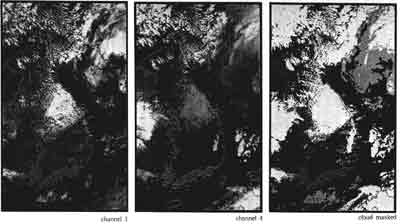
Figure 2: The enhanced image of channel 1 & 4(April 17, 1997) and cloud detection result.
We analyzed sensitivities of the final results for the various thresholds and composting periods (Fig. 3). The final results of our algorithms were very stable to the thresholds and composting period changes although the cloud- masked portions of each step were more or less changed. We investigated the percentage of cloud-free pixels for April 15 to June 30 using the dynamic composting period from 5 to 15 days. It was shown that 10-day was proper composting period to the Korean peninsula but correction to the cloud contaminated pixels composting to be needed.
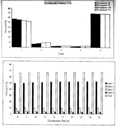
Figure 3: The ratio of cloud contaminated pixels according to the various thresholds and compositing periods
Reference
- Derrien M., B. Farki, L. Harang, H. LeGleau, A. Noyalet, D. Pochic and A. Sairouni, 1993, Automatic cloud detection applied to NOAA-11/AVHRR imagery. 46, 246-267.
- Desbois, M.G. Seze and G. Szejwach, 1982, Automatic classification of clouds on meteosat imagery: application to high level clouds. J. Appl. Meteor., 21, 401-412.
- Ebert, E., 1987, A patern recognition technique for distinguish surface and cloud types in the polar regions. J. Clim, Appl. Meyoer., 26, 1412-1427.
- Inoue, T., 1985, On the temperature and effective emissivity determination of semi-transparent cirrus clouds by bi-spectral measurements in 10mm window region. J. Meteor. Soc. Japan, 63,88-98.
- Inoue, T., 1987, Acloud type classification with NOAA-7split-window measurements. J. Geophys. Res., 92, 3991-4000.
- Planet, W.G., 1988, Data extraction and calibration of Tiros-N/NOAA radiometers, NOAA Technical Memorandum NESS 107, Washington, D.C.
- Reynolds, D.W and T.H. Vonder Haar, 1977, A bi-spectral method for cloud parameter deterination. Mon. Wea. Rev., 105, 446-457.
- Rossow, W.B., 1988, Preliminary documentation for ISCCP C1 data. 1-13.
- Saunders, R.W., and K.T. Kriebel, 1988, An improved method for detecting clear sky and cloudy radiances from AVHRR data. Int. J. Remote Sensing, 9, 123-150.
- Schiffer, R.A. and W.B. Rossow, 1983, The ISCCP: The first project of the world climate research programme. Bull. Amer Meteor. Soc., 64, 779-784.
- Seze, G. and M. Desbois, 1987, Cloud cover analysis from satellite imagery using spatial and temporal characteristics of the data. J. Climate Appl. Meteor., 26, 287-303.
- Simpson, J.J., and J.I. Gobat, 1996, Improved cloud detection for the daytime AVHRR scenes over land. Remote Sens. Enviorn 55,21-49.
- Suh, M.S., and K.Y. Park, 1993, Cloud cover analysis from GMS/S-VISSR imagery using bispectral thresholds technique. J. Korean Soc. Remote Sensing, 9,1-19.