GISdevelopment.net ---> AARS ---> ACRS 1997 ---> Poster Session 1 Graphical Analysis of Spectral Reflectance Curve Nguyen Dinh Duong Institute of Geography , National Center for Natural science and technology of Vitnam Nghiado , Tuliem , Hanoi, Vietnam Fax: 84-4-8361192, 84-4-8352483 E-mail : duong@igg.ac.vn Abstract In the paper the author describes a proposal of an algorithm for automatic classification of multispectral data set . this algorithm called as GASC is being developed under the NASDA ADEOS -II GLI Research Announcement of classification of sex 250m channels of future GLI sensor. Unlike the traditional classification methods that are based on either supervised or unsupervised ( clustering ) principles this algorithm will use graphical invariant such as shape of spectral reflectance curve, angles, area of geometric entities to define features of each land cover object. In case of using Normalised radiance this algorithm offers possibility to automate classification that is very important in processing of huge volume of data observed by sensor Global imager ( GLI) on board of future ADEOS-II satellite. The target of the paper is to explain the nature of the algorithm and to demonstrate preliminary result using LANSAT TM data. Introduction Nowadays Earth remote sensing ahs become increasingly developed and widely utilized due to advancement of technology and the need Earth environment monitoring form space . while the third generation of remote sensing satellite that is featured by very high spectral resolution ( up to 3 or 2 meters ) is already on the horizon and open a new phase of Earth observation in detail the need of global earth observation does not lose its significance but increases from day to day. This urgencies driven by recent learning of environmental degradation caused by growing population and over-exploitation of natural resources. In order to understand what is happening on the earth it is necessary to collect major geophysical parameters that are important for understanding the Earth's environment. The future ADEOS-II program with Global Imager sensor ( GLI) is one of missions targeted to fulfil this aim . it was designed to contribute important information to understanding the carbon cycle, estimating primary biomass production, understanding the energy and hydrological cycles and understanding the change in surface processes due to global warming ( Sciences on GLI Mission -NASDA). GLI sensor on board ADEOS-II with 36 spectral channels covering the spectral range from 0.38 to 12 micron with 1600 km swath and 1km and 250m spatial resolution will generate huge information volume( about 394 MB per scene level -1 A product with 250 m resolution and 129 MB per scene for level-1 A product with 1 km resolution- Fujitsu Report of level 1 and Products Description ) its processing and analysis will be time consuming and requires very big computer resource, in this paper the author submit and algorithm for automatic vegetation and land cover classification using six 250m channels of GLI sensor. This algorithm is developed and tested using a data set simulated by LANDSAT TM data. This is preliminary result of research that is being undertaken in the framework of NASDA ADEOS-II Research Announcement . Graphical analysis of spectral reflectance curve The nature of GASC algorithm is to find out spectral invariant that will help to easily classify land cover objects according to their spectral reflectance characteristics. This method assumes that different land cover objects has different spectral reflectance pattern. This pattern should be stable for certain remote sensing senor with fixed observation spectral channel composition. The six 250m spectral channels of GLI sensor are equivalent to six channels of well known LANDSAT TM sensor excluding the thermal one. Given a pixel vector. P ( b1, b2, b3, b4, b5, b6) b1 Normalised atmospherically corrected digital count of channel 1 b2 Normalised atmospherically corrected digital count of channel 2 b3 Normalised atmospherically corrected digital count of channel 3 b4 Normalised atmospherically corrected digital count of channel 4 b5 Normalised atmospherically corrected digital count of channel 5 b6 Normalised atmospherically corrected digital count of channel 6 then is spectral reflectance curve can be constructed as follows : Figure 1: Definition of spectral reflectance curve This curve can be than described by some graphical invariant. It is possible to establish three invariant group. Invariant group I: this group consists of only one invariant. This is shape or modulation of the spectral reflectance curve. This invariant is defined by 15 parameters that simulate modulation of spectral curve. These 15 parameters are defined as follows. Mij Relation between band j and band I, I= 2,3,4,5,6 and j= 1,2,3,4,5 The value Mij is assigned 1 when bi<bj, 2 when bi= bj and 3 when bi>bj. from theoretical point of view, there would be 3 power 15 possible combinations of Mij. If we assign each combination one integral value then this value will range form 0 to 14348907. in practice the number of combination is far less this value. Generally, for n channel data set we need 9n(n-1)/2 parameter to define the modulation of spectral curve. If this invariant will be used for image classification then the number of categories will be 3 power (n(n-1)/2 in maximum number of spectral reflectance curve patterns depends very much on geometric correction processing. The best result will be obtained with nearest neighbor resampling while other method based on interpolation will falsely increase number of spectral reflectance curve patterns Invariant group II: there group is composed of several invariant that are defined as angles among different segments of spectral reflectance curve. For example angle a on figure 2 can be considered as one of the invariant. 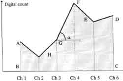Figure 2: Definition of invariant Invariant group III: there are several values that may be used as invariant of this group. They are : bands ratio , indices ….. The author has tried with the following values: - Normalised vegetation index to classify vegetation coverage. - Area of the polygon limited by the spectral reflectance curve and x-axis ( doted area on the figure 2). Classification example To demonstrate the proposed algorithm, the author used a window of LANDSAR TM scene 127/45 observed on 16 October 1996 with 6 channels. The channel 6 stands of the original TM channel 7. the size of the window is 1024 pixels x 1024 lines . on figure 3 is false colour composite of the study are RGB= 432. the study area cover the Hanoi city and vicinity. Land cover of this are is featured by major categories as built up area, water body, paddy field, bare soil and their mixture. The target of the research is to carry out implementation of the proposed algorithm. The author has wrote program composed of Microsoft Visual C 4.0 and FORTRAIN Power station 4.0 modules under windows 95 operating system environment for classification of the extracted window. 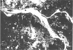The computation in divided into the following steps: Figure 3: False colour composite of the study area Image encoding to get look up table of all unique pixel vectors . Classification of LUT to find out all spectral reflectance curves patterns within the images . Classification of spectral reflectance curve by GASC algorithm If number of patterns is more than 256-> reduction by using frequency value to achieve one bytes classified image If we will take into account only spectral reflectance patterns with frequency higher than 5 then number of patterns of this window is 171. due to code system one is relative and the other is absolute. The relative code of each spectral reflectance patterns ranges from 0 to 255 and changes from image while the absolute code ranges from 0 to 14348907 and is unique for each land cover category. On the figure 3 is false colour composite of the study area and figure 4 shows example of classification using GASC algorithm. This classification example shows possibility to separate land cover categories by using only modulation of the spectral reflectance curve as classification rule. 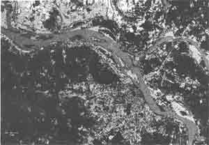Figure 4: Image classified by GASC algorithm The classified image can be interpreted legend as below. - clear water body dark blue colour - turbid or shallow water light blue colour - vegetation with moderate coverage, rice, crop light green colour - vegetation with dense coverage dark green colour - mixture of built up area and trees brown colour - sandy flat cyan colour - built up area or bare surface red colour - bare agriculture soil Yellow colour graphical presentation of major land cover groups can be seen on Table I. Table 1 Code Spectral reflectance curve pattern Dominant land cover 0 111111111111111 Clear water 163296 111133133111111 Vegetation 1239858 113133333313311 Bare surface Conclusion This is preliminary research result of application of GASC algorithm for sex spectral channel data set of LANDSAT TM sensor simulated for the GLI sensor of the future ADEOS-II satellite. The results pointed out possibility to use modulation of spectral reflectance curve as one of data feature for multispectral classification to separate vegetation, water and bare surface. Since there is many mixtures among water, vegetation and bare surface so the use of the other invariant will help to further refining classification and decomposition of mixed land cover categories. Current research point out that it is needed to developed different invariant set for different land cover group . selection of right invariant set for classification is target of next research that requires both algorithm development and ground truth data collection for algorithm validation. Acknowledgement The author thanks NASDA ADEOS-II project for the sponsorship to undertake this research. The author expresses also acknowledgment to fundamental Research program of Vietnam and Institute of Geography, NCTS of Vietnam for supporting this research. Reference: Kalensky, Z.D., 1996. regional and global Land cover Mapping an environmental Monitoring by Remote sensing, Proceeding, XVIII ISPRS Congress, Commission IV, working group 6. science on the GLI Mission March 1996. Fujitsu Report of Level 1 an Products Description, the second ADEOS-II/GLI workshop, June 1997, Kinugawa Onsen, Japan . Nguyen dinh Duong, ADEOS-II/GLI RA interim progress of research " Vegetation and land cover classification based on simulated GLI multitemporal data sets ".