| GISdevelopment.net ---> AARS ---> ACRS 1997 ---> Poster Session 1 |
Computer Analysis of Spatial-
Temporal Organization of Structure Landscapes of the Azerbaijan Republic
Nabiyev Alipasha
Alibek
Baku state University, Department of Physical Geography
Faculty of Geography 370148 Baku, Z.Khalilov street, 23.
Abstract Baku state University, Department of Physical Geography
Faculty of Geography 370148 Baku, Z.Khalilov street, 23.
At present stage of physical geography development mainly the paleogeography is required for quantative analysis with applying of computer, so that this analysis allows to have acces for application of complex modern mathematic models such as theory of combinations , nonparametric and parametric mathematical-statistic methods, by which are succeed to discover more disctintive pecularities in structure and development of paleolandscapes. The results is invaluable on the regional geosystem forecasting .
Introduction
In this work for the first time in Azerbaijan is applying complex methods of modern mathematics so called matrix computation in the plaeolandscape investigation s of description of more practicable structure and their characteristic elements such as determination of structure's and interrelation of structural elements of geographical complexes with the alteration of leadership in time.
The investigation of paleolandscapes spatial-temporal structure by means of mathematic-cartographic modelling on computer IBM PC 586 if quantitative elements of the paleolandscapes structure are taken form the Azerbaijan Republic paleolandscapes maps, which compiled by prof M.A.Museibov (1981) for nine sections of geological time. I. Upper Miocene, II . Middle Pliocene, III. Upper Plioncene ( agchagil century ), IV. and absheron century ), IV Under Pleistocene ( Baku centurly), Middle Pleistocene ( Gurgans century (IV), Caspian century (VII), khvalyn century (VIII)),. IX. Late Pleistocene ( The end of Khvalyn century ), and X. Holocene (Modern century ).
The Methods of Research and Results
For solution of this problem with some modification which connected with character of investigation we have took the method, suggested by A.G.Topchiyev (1979) and the methods mathematical-system analysis.
The work have been carried out by following stages.
1. Matrix analysis of plaeolandscapes neighbourhood ( meeting )
The goal of this analysis is to determone the leading paleolandscapes which are the core of paleolandscapes general structure and this period of the considering region.
The second to determine secondary elements in the paleolandscapes structures of investigated region at this period, so called core satellite of paleolandscapes structure. To define these elements of paleolandscapes structure the A.G.Topchiev's criteria in interpreted as follows:
a) Natural Complexes (NC) is appeared as one of the landscape's structure score if
b) Natural complexes appears as a satellite ( non leading ) of one or some different cores if
c) Natural Complexes has a boundary distribution which is closed to incident if
For solution of this question we have determined occurrence number of plaeolandscapes in space on the paleolandscape maps of Azerbaijan. On this bases have composed the matrix of occurrence, which have determined A.G.Topchiev's criteria values.
Result Example
| \N \N |
1 | 2 | 3 | 4 | 5 | 6 | 7 | 8 | 9 | 10 | 11 | 12 | 13 | 14 | Sum(i) | T(i) |
| 1 | 0 | 3 | 2 | 0 | 1 | 0 | 0 | 0 | 0 | 0 | 0 | 0 | 0 | 0 | 6 | 1.0 |
| 2 | 3 | 0 | 3 | 1 | 0 | 0 | 0 | 2 | 0 | 0 | 1 | 0 | 0 | 0 | 10 | 1.2 |
| 3 | 2 | 2 | 0 | 1 | 1 | 0 | 1 | 1 | 1 | 1 | 0 | 0 | 0 | 0 | 10 | 0.9 |
| 4 | 0 | 1 | 1 | 0 | 0 | 0 | 0 | 0 | 0 | 0 | 0 | 0 | 0 | 0 | 2 | 1.0 |
| 5 | 1 | 0 | 1 | 0 | 0 | 0 | 1 | 0 | 0 | 0 | 0 | 0 | 0 | 0 | 3 | 1.0 |
| 6 | 0 | 0 | 0 | 0 | 0 | 0 | 0 | 0 | 1 | 1 | 0 | 0 | 0 | 0 | 1 | 1.0 |
| 7 | 0 | 0 | 1 | 0 | 0 | 0 | 0 | 0 | 1 | 1 | 0 | 0 | 0 | 0 | 2 | 1.0 |
| 8 | 0 | 1 | 1 | 0 | 0 | 0 | 0 | 0 | 0 | 0 | 1 | 0 | 0 | 0 | 3 | 0.7 |
| 9 | 0 | 0 | 1 | 0 | 1 | 0 | 0 | 0 | 1 | 1 | 0 | 0 | 0 | 0 | 3 | 1.0 |
| 10 | 0 | 0 | 1 | 0 | 0 | 1 | 1 | 0 | 0 | 0 | 0 | 0 | 1 | 0 | 5 | 1.0 |
| 11 | 0 | 1 | 0 | 0 | 0 | 0 | 0 | 1 | 0 | 0 | 0 | 1 | 1 | 0 | 4 | 1.0 |
| 12 | 0 | 0 | 0 | 0 | 0 | 0 | 0 | 0 | 0 | 0 | 1 | 0 | 0 | 3 | 4 | 1.0 |
| 13 | 0 | 0 | 0 | 0 | 0 | 0 | 0 | 0 | 0 | 1 | 1 | 0 | 0 | 0 | 2 | 1.0 |
| 14 | 0 | 0 | 0 | 0 | 0 | 0 | 0 | 0 | 0 | 0 | 0 | 3 | 0 | 0 | 3 | 1.0 |
| SUM(j) | 6 | 8 | 11 | 2 | 3 | 1 | 2 | 4 | 3 | 5 | 4 | 4 | 2 | 3 |
According to the results of the Topchiev's criteria t(i) we have composed the landscapes organization maps which reflected leading ( core structure ) and subordinate ( care satellites-landscapes ) elements at the paleolandscapes structure ( organization).
The analyses of he pleolandscapes organization maps have discovered that:
- T the leading paleolandscapes are not meeting at the Upper Miocene . it shoves that the paleolandcsape structure core not formed at this period so all the paleolandscapes have lead accidentally distributed character .
- At the Akchagil centrury the cores composition is continned to become complicated. Some of middle mountains and plain landscapes are characterized by accidental distribution.
- At the Baku century the middle mountains an plain paleolandscape are gone out of the core satellites composition and become of paleolandscape structure core. On this case at this century have created contrast and the paleolandscape structure.
- At the Caspian century height mountainous and middle mountainous paleolandscape have gone out of the composition of core and become accidentally distributed elements of structure. The structure core of paleolandscape at this century were plain and middle mountains paleolandscape
- At khvalyn century high mountainous and middle mountains paleolandscape have returned to the composition of ht core's satellites. The core of paleolandscape structure consisted of plain, foot mountainious and some where middle mountainous paleolandscape .
- At the end of khvalynian century the core of paleolandscape structure consisted from plain, foot mountainous, middle mountainous and high mountainous paleolandscapes.
By the A.G.Topchiyev's neighborhood differences.
To establish and quantitatively cost relations predominate subordination for every pair of elements of landscape structure. The sum of positive and negative differences are using for systematic of landscapes structure elements by their appearance in spatial structure' Criteria's of systematic were these conditions .
- summer of negative neighborhood of differences shows, that these paleolandscape are dominants in spatial organization, so that they appears as main elements of paleolandscape structure.
- Sums of positive neighborhood differences shows that these paleolandscape are sub dominates so that they are subordinate elements of this landscape structure.
- The elements of paleolandscape structure with zero neighbourhood difference is characterized accidental distribution.
Result Example
| \N\N\ | 1 | 2 | 3 | 4 | 5 | 6 | 7 | 8 | 9 | 10 | 11 | 12 | 13 | 14 | SUM(-) | SUM(+) |
| 1 | 0 | 0 | 0 | 0 | 0 | 0 | 0 | 0 | 0 | 0 | 0 | 0 | 0 | 0 | 0 | 0 |
| 2 | 0 | 0 | -1 | 0 | 0 | 0 | 0 | -1 | 0 | 0 | 0 | 0 | 0 | 0 | -2 | 0 |
| 3 | 0 | +1 | 0 | 0 | 0 | 0 | 0 | 0 | 0 | 0 | 0 | 0 | 0 | 0 | 0 | +1 |
| 4 | 0 | 0 | 0 | 0 | 0 | 0 | 0 | 0 | 0 | 0 | 0 | 0 | 0 | 0 | 0 | 0 |
| 5 | 0 | 0 | 0 | 0 | 0 | 0 | 0 | 0 | 0 | 0 | 0 | 0 | 0 | 0 | 0 | 0 |
| 6 | 0 | 0 | 0 | 0 | 0 | 0 | 0 | 0 | 0 | 0 | 0 | 0 | 0 | 0 | 0 | 0 |
| 7 | 0 | 0 | 0 | 0 | 0 | 0 | 0 | 0 | 0 | 0 | 0 | 0 | 0 | 0 | 0 | 0 |
| 8 | 0 | +1 | 0 | 0 | 0 | 0 | 0 | 0 | 0 | 0 | 0 | 0 | 0 | 0 | 0 | +1 |
| 9 | 0 | 0 | 0 | 0 | 0 | 0 | 0 | 0 | 0 | 0 | 0 | 0 | 0 | 0 | 0 | 0 |
| 10 | 0 | 0 | 0 | 0 | 0 | 0 | 0 | 0 | 0 | 0 | 0 | 0 | 0 | 0 | 0 | 0 |
| 11 | 0 | 0 | 0 | 0 | 0 | 0 | 0 | 0 | 0 | 0 | 0 | 0 | 0 | 0 | 0 | 0 |
| 12 | 0 | 0 | 0 | 0 | 0 | 0 | 0 | 0 | 0 | 0 | 0 | 0 | 0 | 0 | 0 | 0 |
| 13 | 0 | 0 | 0 | 0 | 0 | 0 | 0 | 0 | 0 | 0 | 0 | 0 | 0 | 0 | 0 | 0 |
| 14 | 0 | 0 | 0 | 0 | 0 | 0 | 0 | 0 | 0 | 0 | 0 | 0 | 0 | 0 | 0 | 0 |
At result of these matrix we followed elements of paleolandscape structure by their appearance in spatil structure. Composed the maps of dominate and subdominate elements of paleolandscape structure.
3. Matrix analysis of positional resemblance
Matrix of positional resemblance was computed on the base of species and individual resemblance matrix with the help of hemming measures, which look as follows.
| P(i,j)= | N(i,j) ------------------------- N(i)+n(j)-n(i,j) |
Where n(i0, n(j)-number of neighbours "i" and "j" natural complexes: but n(i,j) the number of common neighbors., computing examples ( table .3).
| Species NC | number of individual contour of landscape | |||||||||||||
| 1 | 2 | 3 | 4 | 5 | 6 | 7 | 8 | 9 | 10 | 11 | 12 | 13 | 14 | |
| Si (2) | 1 | 0 | 1 | 1 | 0 | 0 | 0 | 1 | 0 | 0 | 1 | 0 | 0 | 0 |
| Si (3) | 1 | 1 | 0 | 1 | 1 | 0 | 1 | 1 | 1 | 1 | 0 | 0 | 0 | 0 |
Common neighbors +-----------+----------+--------------------------------
(here data taking of Table 1)
The value of positional resemblance is changed in the limits of 0-1 and can be interpreted as follows:
| 1. The high resemblance | 0,6 <=p(I,j) <=1.00 |
| 2. Average resemblance | 0,30 <=p(I,j)< 0,60 |
| 3. Low resemblance | 0,00 <=p(I,j) <0,30 |
Computation Example
Matrix of positional resemblance for Middle Pliocene (II)
| 1 | 2 | 3 | 4 | 5 | 6 | 7 | 8 | 9 | 10 | 11 | 12 | 13 | 14 |
| 1 | .14 | .22 | .33 | .20 | .00 | .25 | .50 | .50 | .14 | .16 | .00 | .00 | .00 |
| 2 | .30 | .16 | .16 | .00 | .16 | .16 | .14 | .14 | .12 | .16 | .16 | .00 | |
| 3 | .11 | .11 | .12 | .11 | .10 | .11 | .09 | .10 | .00 | .11 | .00 | ||
| 4 | .25 | .00 | .33 | .66 | .25 | .15 | .20 | .00 | .00 | .00 | |||
| 5 | .00 | .25 | .20 | .15 | .00 | .00 | .00 | .00 | .00 | ||||
| 6 | .50 | .00 | .33 | .00 | .00 | .00 | .50 | .00 | |||||
| 7 | .25 | .33 | .16 | .00 | .00 | .33 | .00 | ||||||
| 8 | .20 | .14 | .16 | .25 | .25 | .00 | |||||||
| 9 | .14 | .00 | .00 | .25 | .00 | ||||||||
| 10 | .12 | .00 | .00 | .00 | |||||||||
| 11 | .00 | .00 | .25 | ||||||||||
| 12 | .33 | .00 | |||||||||||
| 13 | .00 | ||||||||||||
| 14 |
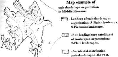
Map example of paleolandscape organization in Middle Pliocene.
On basis the table 4 and interpretation we have lined out gramped and weekly connected elements of paleolandscapes structure of the investigated region. These structural interrelations are presented as color graph-model, which showed all characteristics of positional resemblance NC.