| GISdevelopment.net ---> AARS ---> ACRS 1997 ---> Global Environment |
Satellite Land Surface
Temperature for Sarawak Area
Hadi Batatia1
and nabil Bessaih2
Managing Director
University Malaysia Sarawalk
94300 Kota Smarahan
Sarawak - Malaysia
1Tel: + 60 82671000 Fax: + 60 82672301
E-mail :bessaih@feng.unimas.my
2Tel: + 60 82671000 Fax: 60 82672317
E-mail :bessaih@feng.unimas.my
Abstract
Managing Director
University Malaysia Sarawalk
94300 Kota Smarahan
Sarawak - Malaysia
1Tel: + 60 82671000 Fax: + 60 82672301
E-mail :bessaih@feng.unimas.my
2Tel: + 60 82671000 Fax: 60 82672317
E-mail :bessaih@feng.unimas.my
Land Surface Temperature is a key parameter in many remote-sensing applications. This temperature can be estimated from rremotely sensed infrared radiance. Two major phenomena have direct effects on the infrared radiance received by the satellite, namely atmospheric effects and surface emissivity. Many algorithms have been developed to take into account these effects. This paper presents the results of a study that aimed to evaluate the importance of these effects in the region of Northern Borneo. The study consisted in the implementation of an algorithm that corrects water vapour and emssivity effects on the estimated land surface temperature. This algorithm uses the split window method, which consists in measuring the temperature using two different infrared channels, and eliminating the effect between these two measurements. Uncorrected and corrected land surface temperature maps were determined for the region under study. These maps show the importance of the surface emissivity and atmospheric effects. The study suggests an accurate estimation of water vapour profile and emissivity in order to estimate accurately land surface temperature.
Introduction
Land Surface Temperature is a key parameter in energy budget models, evaportanspiration models (Serafini, 1987; Bssieres, 1995), estimating soil moisture (Price, 1980), forest detection and forecasting, monitoring the state of the crops, studing land and sea breezes and nocturnal cooling.
Land Surface Temperature can be determined by measuring the radiation emitted by the earth's surface. This radiation will be converted into temperature brightness using the inverse of Planck's radiation equation. Unfortunately, land surface does not behave as a blackbody. The radiation measured by the satellite radiometer include also radiation emitted by the atmosphere and radiation reflected by the land surface. Gases and suspended particles in the atmosphere and radiation reflected by the land surface. Gases and suspended particles in the atmosphere may absorb radiation emitted from objects, resulting in a decrease in the energy reaching a thermal sensor. Scattering, in the presence of suspended particles, can also attenuate ground signals. Atmospheric absorption and scattering tend to make the signals from ground objects appear colder than they are. For this reason, measurement are usually made in two atmospheric absorption free regions (windows ) of the electromagnetic spectrum lying between 3.5mm to 3.9 mm and 10mm to 13mm. Unfortunately, in this spectrum regions, there is residual gaseous absorption, mainly by water vapour. Sobrino et al, (1991), reported that the difference between the real Land Surface Temperature and the satellite surface temperature is of 7oC for a tropical atmosphere. By using a second infrared measurement, either at a different wavelength or at different zenith angle, it is possible to improve the estimation of the surface radiant temperature.
Split window method
The method widely used for correcting the water vapour effects is the split window method. This method makes use of the observation that the transmission of a path trough a most atmosphere at one wavelength is closely correlated with the transmission through the same path at a second nearby wavelength. The advanced very high resolution radimeters (AVHRR) on board of the NOAA 14 satellite employs two channels in the infrared windows between 10mm and 13mm which can be used to exploit this differential effect.
Price (1980,1984), sobrino et al (1991), vidal (1991), Ottle and Vidal-Madjdar (1992), prata (1993) developed split window algorithms, which have global form with coefficients that depends upon local conditions. These algorithms have the following general form:
where,
T0 : real Land Surface Temperature
T4 : channel 4 brightness temperature
T5: channel 5 brightness temperature
A and B are coefficients which depend on the surface emissivities, atmospheric absorption coefficients and total water vapour amount (Sobrino et al, 1991)
Data analysis
Sarawak occupies a large proportion of the northern part of Borneo island. It is located within the longitudes E110o to E114o and N1o to N5o. Over this area cloud cover is frequent. This makes selection of data sets for analysis a tedious task. Ten NOAA-14 AVHRR GAC data sets occurring during June and July 1996 near 5:00 UCT (12:00 LST), which are close to the "midday" conditions required by many applications, have been acquired for this investigation. The satellite data were mapped to UTM projection by using ERMAPPER(™) image processing software. Satellite counts were converted into measured radiance for the five NOAA-AVHRR channels using methods provided in the "NOAA Polar Orbiter Data User Guide".
The radiance measured by channel 3, 4 and 5 were converted to brightness temperature using the equations provided in Kidwell (1995).
For channels 1 and 2, the percent albedo measured by the sensor were converted to spectral radiance using the method described in Kidwell (1995).
Normalised Difference Vegetation Index (NDVI) values were calculated using visible channel (CH1) and near -infrared channel (CH2) reflectance values (Eq.2),
| NDVI = | CH2
-CH1 ------------------- CH2+CH1 |
(2) |
Applying a threshold on the NDVI maps identified the cloudy regions. The cloudy pixels were then eliminated from the Temperature Brightness maps. It was notices that cloudy pixels had brightness temperature lower than 13oC, which is acceptable for the region.
The cloud-free maps for channel 4 and 5 wee overlaid with a map containing land regions. An emissifity of value 1 was to all non-land regions. An emissivity of 0.98 was assigned to all land pixels. The sobrino algorithm (eq.1) was then applied to correct the temperature.
Result and Discussions Figure 1 shows channel of a data set used in this study. This partial set cover the area located within latitudes 0:30N to 7:15N and longitudes 108:30E to 120:30E. Figure 2 presents the NDVI map obtained from this data set. In his map, black pixels have values greater than zero. We notice that clouds are readily identifiable, and that water areas have the minimum values.
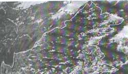
Figure 1: Channel 1 from a data set used in this study
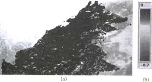
Figure 2. (a) NDVI map obtained from the data set shown in Figure 1. (b) Pseudo-colour scale used to represent the NDVI values.
Considering the land as a black body (emissifity =1), the land surface temperature calculated without atmospheric corrections from channel 4 and 5 are mapped in figures 3 and 4, respectively. Comparing these two maps, we notice a slight difference. This difference is in the range of 0oC to 10oC, with a mean of 4.4oC.
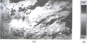
Figure 3. (a) Surface temperatures obtained from channel 4 without taking into accounts emissivity and vapour. (b) Pseudo-colour scale used to represent the temperatures.
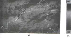
Figure 4. (a) Surface temperatures obtained from channel 5 without taking into accounts emissivity and vapour. (b) Pseudo-colour scale used to represent the temperatures.
After applying the correction algorithm (Eq. 1), we obtain the map presented in figure 5. Observing this map, we can see that the temperatures are higher than those in figure 3 and 4. The difference between the corrected temperatures (fig. 5) and either non-corrected temperatures (fig. 3 or 4) varies between 7oC and 13oC, with a mean of 10oC. This significant difference is obviously due to the effects of water vapour and land surface emissivity.
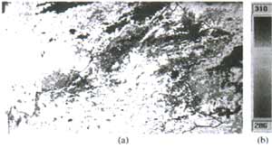
Fig.5 (a) Corrected surface temperature. This map is the result of applying Sobrino algorithm. (b) Pseudo-colour scale used to represent the temperatures.
Further more, we observe that corrected land surface temperature (fig.5) is higher in coastal areas and regions with lower NDVI values (fig. 6). This means that land surface temperature is closely correclated to the land cover especially to the type of vegetation. Hence the importance of the effects of emissivity on land surface temperature.
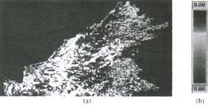
Figure 6. (a) NDVI map for the land areas only. NDVI values lower than 0 (water and cloud regions) are all represented in blue. (b) Pseudo-colour scale used to represent NDVI values.
Conclusion
Estimating land surface temperature is useful for many applications. This study has shown that the effects of water vapour and emissivity on this temperature are important over a tropical region like northern Borneo. We have also noticed that over this region, distinguishing land and water areas is not possible using surface temperature. In addition, land surface temperature was found to be constantly varying in the range of 23oC to 33oC, which is an expected result for the region. However, the results of this study suggest that, in order to develop an accurate model for land surface temperature in this region, we should further investigate the following.
- Estimate water vapour profile using remotely sensed data.
- Estimate water vapour profile using remotely. Correlating the NDVI with the emissivity is one possible and promising way to perform this estimation.
- One major characteristic of the area of interest is the frequent cloud cover. For certain type of applications (e.q. environmental), the cloud problem can be overcome using land surface temperature history and a spatial dependency model. Such technique allows the estimation of temperatures for cloudy pixels by propagating the effects of neighbouring non-cloudy pixel. For applications that require accurate estimation of land surface temperature for each pixel (e.g. real time control), microwave should be used instead of infrared.
- Bussieres, N., (1995). Preliminary Analysis of AVHRR Brightness temperature for evaportanspiration estimation over the Mackenzie Basin Summer 1994. Proceedings of the seventeenth Canadian Symposium on Remote Sensing, Saskatchewan, Canada, 13-15 June 1995.
- Bussieres, No., Louie, P.Y.T, and Hogg, W., (1990). Progress report on the implementation of an algorithm to estimate regional evaportanspiration using satellite data. Proceeding of the workshop on applications of remote sensing in hydrology, Saskaton Saskatchewan, 13-14 February 1990.
- Ottle, C., and Vidal-Madjdar, D., (1992). Estimation of land surface temperature with NOAA 9 data. Remote Sensing Environ., 40, pp. 27-41.
- Prata, A.J., (1993). Land Surface temperature derived from the advanced very high-resolution radiomether and the along-track scanning radiometer. Journal of Geophysical Research, 9, pp. 16689-16702.
- Price, J.C., (1990). The potential of Remotely Sensed Thermal Infrared data to Infer Surface Soil Moisture and Evaporation. Water Resources, 16, pp. 787-795.
- Price, J.C., (1984).; Lnad Surface tempeature measurements from the split window channels of the NOAA-7/avhrr. Journal of Geophysical Research, 89, pp. 7231-7237.
- Serafini, V.V., (1987). Estimation of the evapotranspiration using surface and satellite data. International journal of remote sensing, 8,pp. 1547-1562.
- Sobrino, J.A., coll, C., and Caselles, V., (1991). Atmospheric Correction for land surface temperature using NOAA-11 AVHRR channels 4 and 5. Remote Sensing Environ., 38, pp. 19-34.
- Vidal, A., (1991). Atmospheric and emissivity correction of land surface temperature measured from satellite using ground measurements or satellite data. International journal of remote sensing , 12(12), pp. 2449-2460.
- Kidwell, K.B., (1995). NOAA Polar Orbiter Data Users Guide. NOAA, Washington, D.C., USA.