| GISdevelopment.net ---> AARS ---> ACRS 1997 ---> GIS |
Spatial Data Annalysis and
GIS Applied to Study the Urban-Rural Linkage in Change Mai-Lamphun Area,
Thailand
Tran Hung, Haja
Andrianasolo and Kaew Nualchawee
Space Technology Applications and Research Program, SERD/AIT
P. O. Box 4, Klongluang 12120, Thailand
Tel : (66-2)-524-6109 Fax : (66-2)-524-5597
E-mail :nrc49832@ait.ac.th
Abstract
Space Technology Applications and Research Program, SERD/AIT
P. O. Box 4, Klongluang 12120, Thailand
Tel : (66-2)-524-6109 Fax : (66-2)-524-5597
E-mail :nrc49832@ait.ac.th
The recent rapid urbanization in Chiang Mai-Lamphun area may have many socio-economic impacts on its rural surroundings, including the redistributing of the rural workforce. This paper presents the use of spatial statistical techniques to simultaneously model physical and socio-economic factors affecting the out-flow of rural workforce in order to understand the region-wide spatial impact of the development. This application example also demonstrates that GIS can be efficient technical bed for spatial data analysis in this kind of regional study.
1. Introduction
As the major growth center for Northern Thailand- "metropolitan area" of Chiang Mai-Lamphun is most distinguishable in the region, embracing districts centers located within about 40 kilometers from the city of Chiang Mai and/or Lamphun municipality. Geographically, the study area is located approximately between Latitude 18°08' N and 19°06'N and Longitude 98°30'E and 99°25', with total area of 5806 km2, Administratively, the study area composes of 10 districts of Chiang Mai province and 6 districts of Lamphun province, resulting in total of 146 sub-districts or tambols (Fig. 1). During the last decade, the area had experienced rapid urban expansion and rapid industrial establishments (Suwan, 1992, Tran, 1997). In the past, as Suwan (1992) showed, Chiang Mai is characterized by scattered small-scale and cottage industry. Most have grown from settlements around administrative headquarters, market centers or important transport mode. From 1986, the Northern Industrial Estate with 87 projects implemented (as of December 1994) was built in Muang Lamphun district. The rapid and unbalanced urbanization could severely distort traditional rural-urban relations, widen urban-rural disparity, aggravated landlessness and rural poverty, which in total present on alarming perspective for future development of the study area. As a result of "push" and "pull" factors in the urban-rural linkages, the rural population tend to look for an employment outside the place of their residence. Thus, the rural labor outflow indicating the job attraction of urban centers as well as the excess of free labor released from the agricultural sector could represent the intensity of urban-rural linkages as a result of regional development.
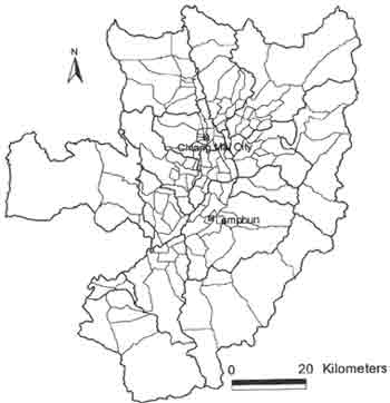
Figure 1. Map of Chiang Mai-Lamphun area with tambol boundaries (lighter lines) and district boundaries (darker lines).
Recent technological advances in geographic information system (GIS) have made it possible to manipulate large amounts of geographic data and construct the topological structure underlying complicated spatial phenomena. The integration of spatial analysis and GIS is an important next step in the development of spatial analysis technologies. Illustrating the importance of integration the technologies, this study is an attempt to model the intensity of urban-rural linkage in Chiang Mai-Lamphun area in terms of intra-regional job distribution in 1994 and to explore the significant socio-economic factors affecting the decision of people to choose place of work. The analyses presented in this paper were conducted on the 'loose coupling' (i.e., using data transfer) between GIS package (Arc/Info 7.0) and spatial statistical software (SpaceStat 1.80).
2. Spatial GIS Database Building and Management
Since the study was emphasizing on macro level of analysis, the data were collected from the secondary sources. The most important source for spatial data is the land-use maps, topographic maps, transportation network map. The major source for socio-economic data were the National Rural Development Database, Ministry of Industry, Chiang Mai and Lamphun provincial offices, Municipality offices, Department of Town and Country Planning, etc.
The spatial data available in forms of paper maps (e.g., land-use, road network maps, etc.) were digitized and introduced into vectors GIS. The digitized maps were corrected and topography was built to make them usable in later analysis. The aspatial (attributes on socio-economic) data were input directly into GIS database and/or converted from database files. The "join" operation was applied to make interrelated information (spatial attributes) combined through a case item. The GIS database for the Chiang Mai-Lamphun project was maintained in Arc/Info 7.0.
3. The Model Specification and Definition of Explanatory Variables
Based on data available at different level and scale, the tambol (sub-district) was chosen as basic areal unit for the study. The spatial overlay and logical-statistical analysis in GIS (Arc/Info) were adopted to summarize the selected information over each areal unit (tambol) for creating the desired spatial variables for the spatial statistical analysis (Tran, 1997).
The percentage of working-out population of each tambol could be served well as indicator for urban-rural linkage and was assumed to be a function of 'push' and 'pull' factors related to demographic, economic and social aspects of development in Chiang Mai-Lamphun area. The spatial data integration in GIS finally produced a set of spatial and spatialized variables for the analysis, which therefore was categorized under three general headings: (1) demographic structure, (2) economic structure, and (3) education attainment. The demographic aspect was represented by population density and the population pressure could be one of the important factors pushing rural people from their village to look for an employment in other places. The social aspect was represented by different level of education attainment (illiteracy, primary education, secondary education) as education was the primary condition for rural people in finding an employment in urban areas (Sriboonruang, 1992).
A large set of economic variables re presenting different economic sectors was submitted to factor analysis in order to identify the underlying dimensions, or factors of economic structure. As result, the economic structure of the study area was represented by 3 major composite economic factors having respective groups of high-factors-loading original variables summarized in Table 1. The detailed procedure to derive 3 major economic factors and their interpretation are beyond the scope of this paper and were discussed in T ran (1997).
- Factor 1(Index of Urban-biased Economy)
high-positively correlates with percentage of urbanized and residential
areas, road density, property taxes and percentage of occupied in
trading population.
- Factor 2(Index of Industrial Economy)highly-positively correlates with total number of industrial employees, number of employees of the large scale factories, number of factories, the total capital investments, the industrial land-use.
- Factor 3(Index of Lacking Opportunity) highly-positively correlates with travel time to nearest town and market centers, median distance to industrial centers and nearest roads, farmer population, and negatively correlates with percentage of agriculture land.
- Factor 2(Index of Industrial Economy)highly-positively correlates with total number of industrial employees, number of employees of the large scale factories, number of factories, the total capital investments, the industrial land-use.
4. Classical Linear Regression Model
In order to avoid the possibility of non-formal errors, the response variable was transformed with a natural logarithm function to create new variable. The transformed variable exhibit a distribution non significantly different from normal at p=0.01, based on Wald statistic. The urban-rural dichotomy played important impacts on most of explanatory variables as shown in Table 2 suggesting that it is necessary to include this important variable (Rural-Urban Indicator) into the starting model. The regression analysis model running under SpaceStat 1.980 software and the insignificant explanatory variables were excluded from models based on t-value (t=0.1). The eventual linear regression model with diagnostic tests was summarized in Table 3.
| Explanatory Variables (units) | F-value | Probability F | Adjusted R-Square |
| Factor 1 | 67.5488 | *0.0000 | *.31458 |
| Factor 2 | 0.0251 | 0.8743 | 0.00677 |
| Factor 3 | 2.40459 | 0.1231 | 0.00960 |
| Illiterate population (%) | 0.8754 | 0.3510 | 0.00086 |
| Primary Educated population (%) | 6.8803 | *0.0097 | 0.03897 |
| Population Density (person/ha) | 58.8338 | 0.0000 | *0.28513 |
| Secondary Educated population (%) | 52.5278 | *0.0000 | *0.26219 |
| Working-out population (%) | 4.2259 | *0.0480 | 0.04117 |
| Response Variable :In (Working-out pop. +1) | ||||
| R2=0.4567 R2-adj=0.4187 Log-likelihood=-101.54 AIC=171.027 | ||||
| Variable | Coefficients | Std. Err. | t-value | Prob |
| Constant | 1.94702 | 0.197472 | 9.859745 | 0.000000 |
| Factor 1 | 0.1777 | 0.100939 | 1.760476 | 0.080511 |
| Factor 3 | -0.452775 | 0.0591491 | -7.60476 | 0.000000 |
| Pop density | -0.000138259 | 5.54217E-05 | -2.494679 | 0.013770 |
| Rural-Urban Indicator | 0.630054 | 0.205611 | 3.064298 | 0.002618 |
| Regression
Diagnostics Multicollinearity condition number = 0.165699 Kiefer-Salmon (error normality) = 11.435 (p = 0.003) Koenker-Bassett test (heteroskedasticity) = 33.138 (p = 0.000) Moran's I (error) = 0.276 (p = 0.000) | ||||
The regression diagnostics showed insignificant non-normal errors and insignificant multicollinearity. However, the spatial autocorrelation was clearly present in the model residual (at significant level of 0.00%), showing significant violation o the basic assumption for linear regression analysis on spatial independence of sampling.
5. Spatial Statistical Model
Because the flow of labor is a spatially dependent process, explanation is not completed without some characterization of spatial intersection. The highly-significantly clustered spatial distribution of working-out population - as shown in Figure 2 and indicated by positive strong Moran's index of 0.4096 and Geary's index of 0.5869 respectively-suggested similar destination and source tambols for labor flows may occur in spatial groups. Inclusion of the spatial lag of response variable -a variable representing the neighborhood effect of the working-out population-may help to explain some of the residual variation. Moreover, the high levels of urban-biased (factor 1) and industrial based economic (factor2) in a tambol not only pull back the local labor, but also attract the additional labor from neighboring tambols. The spatial lags of the factor 1 and factor 2 - representing the 'pull' effects of neighboring tambols -thus, were calculated for each tambol (using adjacency weight matrix) and included as additional explanatory variables into the spatial statistical model. This model, termed the regressive-spatial-autoregressive model (Anselin, 1988) was calculated though maximum likelihood estimation in SpaceStat 1.80 (Anselin, 1995) with results summarized in Table 4. The explanatory variables insignificantly influencing on the realization of the response variable were excluded from the model based on the probability of the z-statistics (using criteria p=0.1). The spatial lag term for response variable was highly significant and, more importantly, its addition reduced the spatial autocorrelation in the model residual to an insignificant level (Table 4). As expected the overall fit of the models were improved with the addition of spatial lag variables: the log-likelihood increased and the AIC significantly decreased (Table 3 & 4). The estimates of the model parameters in the spatial lag model were more precise, i.e., the standard errors of the estimates were lower.
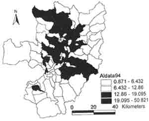
Figure 2 Spatial pattern of working-out population (in %) by tambol in Chiang Mai-Lamphun.
| Response Variable: In(working-out pop. +1) | ||||
| Pseudo R2=0.4921 Log-likelihood=-88.428 AIC=122.855 | ||||
| Variable | Coefficients | Std. Err. | z-value | Prob |
| Lagged | ||||
| Working-out pop. | 1.39591 | 0.232631 | 6.000540 | 0.000000 |
| Constant | 0.0497432 | 0.0126568 | 3.930154 | 0.000085 |
| Rural-Urban Indicator | 0.464627 | 0.187835 | 2.473583 | 0.013377 |
| Factor3 | -0.322413 | 0.0597546 | -5.395623 | 0.000000 |
| Pop. Density | -9.88531E-05 | 5.02207E-05 | -1.968374 | 0.049025 |
| Lagged Factor2 | 0.186305 | 0.105104 | 1.772585 | 0.076297 |
| Regression
Diagnostics Breusch-Pagan (heteroskedasticity) = 36.347 (p = 0.000) Langrange Multiplier test (spatial error dependence)=(p=0.125) | ||||
6. Interpretations and Conclusions
Given the satisfactory diagnostics tests, the relationships between the response and explanatory variables can be interpreted with some degree of confidence. Approximately half of the variation in the working-out population in 1994 is accounted for by the demographic and economic 'push-pull' factors (a reasonably good fit among social science studies). According to the sign of estimated parameters for explanatory determinants and the meaning of the model (Table 4), the significant 'pull' factors were factor 3, factor 2, population density, and significant 'push' factors are rural-urban dichotomy, spatial lag of response variable itself. A closer look at the original economic variables behind factor 3 (Table 1) showed that the accessibility was indeed a crucial factor in providing rural people opportunity to go out for employment, i.e., intensifying the urban-rural interaction. Moreover, the model was also in support of the conventional wisdom that the land pressure was the real force affecting the outflows of free agricultural labor (Table 1). It was found that the population pressure was not a factor affecting the outflow of rural labor. The rural population tend to rushing out to seek for an employment than the urban population as the urban centers were providing good employment opportunity. Concerning the economic factors, the urban-biased economy (factor 1) appeared not significantly affecting the outflows of labor from rural areas, while the industrial-based economy (factor 2) was significantly attracting the rural labor. This findings have more spatial contexts since the urbanization in fact is concentrated mostly around the Chiang Mai city an the rapid industrialization process in the study area since 1986 appeared to have favorable impacts on employment generation for rural population.
In summary, as an important linkage type in the urban-rural interaction, the spatial statistical model of working-out population had provided insights into the mechanism of influences of demographic, economic and social factors upon the outflow of rural labor. In this study, accounting for the spatial association in the data resulted in a spatial model that better extracts information from the variables and has more precise estimates of model coefficients than does the OLS model. By this case study, GIS had proved to be efficient in managing data set (combined both physical and socio-economic spatial variables) for spatial Stastical modeling and for visualization of results for developing and verifying geographical hypotheses.
References
- Anselin L., 1995. SpaceStat, A Software Program for the Analysis of Spatial Data, Version 1.80 Regional Research Institute, West Virginia University, Morgantown, West Virginia.
- Anselin L., 1988. Spatial Econometrics: Methods and Models. Studies in Operational Regional Science. Kluwer Academic Publishers, London
- Sriboonruang S., 1992. Chiang Mai province and its emerging development problems. Faculty of Economics, Chiang Mai University.
- Suwan M., et al., 1992. Impacts of industrialization upon's the village's life in Northern Thailand. Faculty of Social Science, Chiang Mai University.
- Tran Hung, 1997. Integrating GIS with spatial data analysis to study the development impacts of urbanization and industrialization : case study of Chiang Mai-Lamphun area, Thailand. Ph. D. Dissertation, AIT, Bangkok, Thailand (Forthcoming)