| GISdevelopment.net ---> AARS ---> ACRS 1997 ---> Digital Image Processing |
A Combination of a symbolic
and a natural classifier applied to remote sensing images
Case of study: Penang Island
Case of study: Penang Island
Lionel Beauge, Alain
Ketterlin* Ahamad Tajudin Khader, Ruslan Rainis*, Jersy
Korczak*
School of Computer Sciences and *School of Humanities
Universiti Sains Malaysia
11800 USM Pulau Pinang, Malaysia
&
*LSIIT
Department d'Informatique de l'Universite & Louis Pasteur
67084 Strasbourg, France
E-mail : lionel@cs.usm.my
Abstract
School of Computer Sciences and *School of Humanities
Universiti Sains Malaysia
11800 USM Pulau Pinang, Malaysia
&
*LSIIT
Department d'Informatique de l'Universite & Louis Pasteur
67084 Strasbourg, France
E-mail : lionel@cs.usm.my
In remote sensing, images become more and more complex, stemming from the appearance of higher performance satellites. For years, several kinds of formal models have been applied to analyze them, but complex formalisms lead to high computational complexity e.g. morphology mathematical processings. The ongoing research focuses on a hybrid classifier which can discover automatically structured objects on images, in order to generate thematic maps. In this paper, two unsupervised models are presented. The models are based respectively on conceptual classification (the Cobweb algorithm) and on competitive neural network learning to validate our approach. The case of study is Penang Island which provides several kinds of landscape. The resulting maps are quite similar. Our results are also compared with the thematic map of an expert. Our research tend finally toward an hybrid model which integrates symbolic and neural learning, geometrical aspects and expert knowledge. Our main goal is to produce a map updating system whose maps can be used in the studies on environment monitoring e.g. land and urban utilization, vegetation distribution and its changes, regional development etc.
1. Introduction
Remote sensing images provide spectral values about the region under observation. These spectral data allow to distinguish different spectral forms in images by combining all the bands. But images are mote than a simple collection of spectral values. Pixels which are the basic units of the image are also spatially organized. In fact, spectral and spatial values are two kinds of sources of data which can be analysed in different phases or levels and can be combined to obtain the best classification. The goal of classification is to automatically create thematic maps of the region under observation.
2. Methods
2.1 Segmentation principle
Segmentation consists in finding regions or objects that present a thematic meaning regarding to the expert. It is closed to clustering by the fact that it analyses each pixel-element of the image to form a set of distinct classes. In remote sensing, clustering consists in finding a set of classes in the measurement space é = {C1 ,……., Ck) , where C represents the set of all pixels. Each class Ci i e {I,……k} represents a specific subset of the space of spectral a specific subset of the space of spectral values. Objects in the same classes (" : Oj e Ci) have to be similar and objects from different classes have to be sufficiently different. The problem is to find regularities to the measurements space and to produce homogeneous classes. After segmentation, each pixel is assigned to one class only. The set of classes can be organized as a hierarchy or a single set.
2.2 Unsupervised model
Due to the complexity of images and the missing classified data, most of processings tend to be unsupervised. Knowledge is not enough to give information on each pixel of the image.
In this paper, we present two different kinds of classifier which are both unsupervised. The first one is symbolic and takes spectral and based on neural networks and makes at present segmentation based on spectral values only.
3. A conceptual Classifier
3.1 Principles
Our first clustering method is inspired by research in machine learning. The Cobweb algorithm is a generic clustering algorithm which can handle any kind of vector or composite data [2]. Even though it shares several aspects with "classical" statistical algorithms in the context of pixel-based clustering, it also exhibits several distinctive features which make it especially applicable to satellite remote-sensing images analysis.
The first major advantage of Cobweb is that it produces a hierarchy of classes, sorted form the most general to the most specific. This allows a convenient exploration of the classification results, as will be illustrated in our case study. Eventually, it allows the analyst to generate several maps from the same classification result. The second major advantage of this algorithm is that it is incremental, processing one pixel after the other. It is thus able to process very large images without requiring a lot of memory, since it does not need to keep the whole image in memory.
3.2 The Algorithm
The Cobweb algorithm maintains a hierarchy of classes, and updates some classes in this hierarchy any time it gets a new pixel. The first pixel makes a new class by itself, and the second may lead to a new class (if it is different from the first), both of them becoming subclasses of a newly generated root-class. This is enough to bootstrap the process. The next pixels will be driven through the growing hierarchy, starting at the root and following the most adequate path down the tree. Full details of the algorithm are give in [4]. This section provides only the most important assumptions behind Cobweb.
When driving an incoming pixel through the hierarchy, Cobweb tries to adapt the classes to account for the new data. This updating process is twofold. First, several statistics (such as the estimated mean and standard deviation) are compared and stored in each class to provide some descriptive information. Second, the local structure of the hierarchy (i.e. one class along with its sub-classes) is tentatively modified, and the changes are made permanent if they lead to the increase of a heuristic (described below). Those structure modification operators include the creation of a new class covering only the incoming pixel (in which case the algorithm stops, and goes on considering the next pixel), the merging of two sub-classes (by insertion of an intermediate class), or the splitting of one the sub-classes (by promoting this class sub-classes as new direct descendants ) . In each case a new partition is generated at the current level, and this new partition is evaluated. The best possible modification is applied before the algorithm recourses to a deeper level, to continue the incorporation of the pixel. The process stops when reaching a terminal node (a node with no sub-class).
As any clustering algorithm, Cobweb tries to group pixels that are similar, while separating dissimilar ones. This is performed while generating variations of the current partition. Each generated partition is evaluated in terms of the precision of the classes involved. If II (C ) measures the denseness of class C, Cobweb uses the following heuristic to distinguish between candidate partions:
In this formula, C is the main class, which is split into {C1 ,……, Ck} is the proportion of pixels of C affected to Ck. In turn, II (Ck) can be defined as:
Where sik is the estimated standard deviation on spectral values of the ith band for pixels converted by Ck.
This formula can be seen as an average of the gain in precision implied by splitting C into {C1,…., Ck}. By computing the value of this heuristic for each potential partition, Cobweb can select the one with the best score and apply the corresponding update. It thus continually updates the class hierarchy to reflect the data, and keeps a completes range of general to specific classes.
4. A neural classifier
4.1 Principles
Our second clustering method is based on competitive learning as proposed by Rumelhart and Zipser. By training, this unsupervised method allows the neural network to find homogeneous clusters in the input population by self-organization. The network is supposed to discover statistically salient features in the pattern input set.
After learning, each input vector is assigned to one cluster. In a cluster, vectors are similar to each other. Homogeneity of the clusters depends on this similarity between vectors in one class.
The neural network produces one resulting images where pixels are gathered together into classes. This map is considered as a thematic map but without labeled classes. In order to assign a label to each class, expert's knowledge is required.
4.2 Competitive algorithm
The proposed model contains two layers n-m-which are fully interconnected via randomly initialized weights. The input layer contains n neutrons corresponding to the number of components of the input vector. These components corresponds to spectral values of one pixel (x,y) in each image. Each vector is successively presented to the input layer [see figure 1].
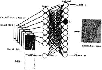
Figure 1: Self-Organizing Neural Net
After propagation of information through the network via connections, the winning output neuron is selected by a 'Winner-takes-all' rule. The following rule describing the minimal distances between the input vector x and the weights of connection which feed into unit i wi. The winner k is the output neuron which possesses the minimal distance:
||.|| denotes the Euclidian norm. Moreover, with this method, there is no need for normalization of the weights and the input data.
The adaptation rule modified weights according to a variation vector:
where the variation vector corresponds to a difference vector:
The parameters a such as 0 £ a <<1, is called the learning rate. The modification of weights can be instantaneous i.e. weights are modified at each time t by the presentation of a new example, or global i.e. after the presentation of all the set of examples. In this case the variation is computed at each time t and the update is done at the end of each presentation of pattern set. Advantages of this latest method are that the order of pixel presentation has no importance and convergence of the network is quicker. [3] [1].
After several presentation of the pattern input set, the network becomes stabilized. Pixels are definitively affected to one specific class and the total square error E which is computed after each presentation of the input set, becomes minimal.

k denotes the unit winning with input xp.
5. Image segmentation
Original images come from Landsat TM and Spot. The region under observation corresponds to an area near the campus of the Universiti Sains Malaysia located on Penang Island. This area has already been analysed by expert. Thematic maps for it has been produced manually. In our case, satellite images has been presented to the previous classifies in order to automatically obtain thematic maps of the region under observation. For reasons of space, we present her only three images obtained with our classifiers from SPOT and Landsat TM satellite images.
5.1 Classified image from the Symbolic classifier
The given image [see figure 2], produced by the conceptual classifier, is obtained with a state of hierarchy of classes which is given in figure 3. Classes are given by the leaves of the tree.
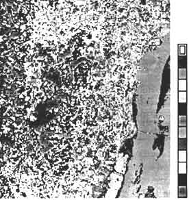
Figure 2: Resulting image (from Spot)
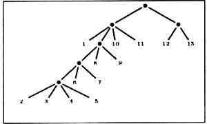
Figure 3: Hierarchy of classes
The thematic images [see figure 2] contains 13 classes. We can recognize different classes for water, vegetation and urban.
5.2 Classified image from the Neural classifier
This result [see figure 4] has been produced by the neural network with an error summation method i.e. with a global variation of weights.
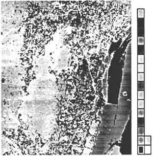
Figure 4: Resulting image (from Spot)
The image [see figure 4] contains 18 classes. We can also recognize classes for urban and roads, for different kinds of water and different kinds of vegetation.
On this image, roads appear distinctly in white color and an area with a high level of town planning is also visible.
The result in figure 5 has been produced by the neural networks with an instantaneous variation of weights from Landsat TM satellite images. The image contains 8 classes. The Penang' bridge and a main road is obviously visible.
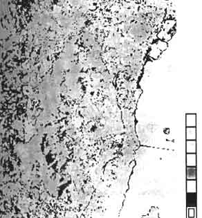
Figure 5: Resulting image (from Landsat TM)
5.3 The landuse map of the expert
The region under observation has been analysed by an expert. It corresponds to an area near the campus of Universiti Sains Malaysia in Penang Island. On the map shown in figure 6, classes are larger and less precise.
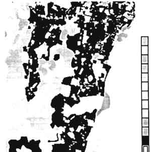
Figure 6: Landuse map of the expert (from Landsat TM)
5.4 Comparisons of the results
The following tabular [see tabular 1 divided into two parts for reasons of space] presents the confusion matrix between the previous results obtained from SPOT images with the symbolic and the neural classifiers.
The 13 classes {C1,….C13} of the image in figure 2 are given in columns and the 18 classes {C1,…..C18} of the image figure 4 are given in lines.
Values represented in matrix correspond to frequences of apparition of a pixel in the two concerned classes.
Even if the number of produced classes - thirteen and eighteen - is not exactly the same to compare, we aim to underline that we can distinguish some quite specific classes in both images. The confusion matrix contains many values at zero and a diagonal line of values appears. So the assignments of pixels into classes with the symbolic and the neural methods give similar results. Some specific classes from both resulting images can be grouped : (C4fig2; C2fig4, C3fig4) ; (C13fig2; C16fig4); (C12fig2; C16fig4, C18fig4).
When we compare our image shown in figure 5 with, the landuse map of the expert, shown in figure 6, the classification give classes which are close together but with more precision: the reclaimed land, the same splitting of Island into two main parts, the same distribution of vegetation etc. According to the expert, the results are meaningful.
| C1 | C2 | C3 | C4 | C5 | C6 | C7 | |
| C1 | 239 | 1276 | 10258 | 973 | 555 | ||
| C2 | 82 | 205 | 12704 | 15663 | 3773 | 3988 | |
| C3 | 317 | 2785 | 592 | 1449 | 103 | ||
| C4 | 437 | 730 | 1635 | 2871 | |||
| C5 | 288 | 1270 | 11115 | 1744 | |||
| C6 | 713 | 970 | 37 | ||||
| C7 | 420 | 7 | 839 | 9182 | |||
| C8 | 683 | 365 | 3153 | 5279 | |||
| C9 | 1076 | ||||||
| C10 | 189 | 1639 | |||||
| C11 | 995 | 1729 | |||||
| C12 | 607 | 1540 | |||||
| C13 | 2 | 2184 | |||||
| C14 | 242 | 646 | |||||
| C15 | 294 | 305 | |||||
| C16 | 516 | 80 | 226 | 1 | |||
| C17 | 20 | ||||||
| C18 | 108 | 6 | |||||
| freq | 3800 | 14652 | 25747 | 16636 | 6648 | 22405 | 19217 |
| C8 | C9 | C10 | C11 | C12 | C13 | freq | |
| C1 | 13301 | ||||||
| C2 | 36415 | ||||||
| C3 | 5246 | ||||||
| C4 | 884 | 1 | 6558 | ||||
| C5 | 14417 | ||||||
| C6 | 4179 | 1980 | 71 | 7950 | |||
| C7 | 6817 | 6 | 17271 | ||||
| C8 | 2249 | 30 | 11759 | ||||
| C9 | 5305 | 4639 | 349 | 11369 | |||
| C10 | 702 | 1833 | 4363 | ||||
| C11 | 360 | 3084 | |||||
| C12 | 2147 | ||||||
| C13 | 324 | 2510 | |||||
| C14 | 55 | 943 | |||||
| C15 | 381 | 980 | |||||
| C16 | 12700 | 4319 | 17842 | ||||
| C17 | 2541 | 2561 | |||||
| C18 | 10746 | 10860 | |||||
| freq | 19434 | 7327 | 2938 | 2977 | 23476 | 4319 | 169576 |
6. Conclusion and orientations
In this paper two kinds of unsupervised classifiers have been presented and applied to SPOT and Landsat TM image segmentation. The algorithm are effective to find clusters in spectral data set and results obtained are meaningful in term of classes.
The classification is fast for small images which size is around 500x500. The next step of our research is to add expert knowledge in order to label automatically our resulting images.
As shown in figure 1 we will also include other kinds of input data such as Digital Elevation Model (DEM) to ameliorate for example the classification of water. This kind of data can be added at a second level of a modular neural network model after a first classification.
A hierarchy of classes for the neural network will also been realized in order to compare and combinate results with the symbolic classifier.
References
- F. Hammadi Mesmoudi. Classifier neuronal d'images de teledetection. PhD thesis, Universite Louis Pasteur, LSIIT, Strasbourg, decembre 1995.
- A. Ketterlin. Decouverle de concepts structures dans les bases de donnes. PhD thesis, Universite Louis Pasteur, LSIIT, Strasbourg, novembre 1995.
- J. Korczak and F. Hammadi-Mesmondi. An Unsupervised Neural Network Classifier and its Application in Remote Sensing. In Proc. Internat. Conf. on Image Processing, Edinbourg, 1995.
- J. J. Korczak, D. Blamont, And A. Ketterlin. Thematic image segmentation by a concept formation. In J. Desachy (ed.), editor, Image and signal processing for remote sensing, volume 2315, Roma, Italy, 1994. SPIE Proceedings Series.