| GISdevelopment.net ---> AARS ---> ACRS 1994 ---> Water Resources |
Runoff Analysis in South East
Asia using DEM and Remote Sensing Data
Masataka TAKAGI and Shunji
MUKAI
Institute of Industrial Science,
The University of Tokyo
7-22, ROPPONGI, MINATO_KU, Tokyo 106,JAPAN
Tel. +81-3-3402-6231
Fax. +81-3-3479-2762
E-mail: mailto:%20murall@shunji.iis.u-tokyo%20ac.jP
AbstractInstitute of Industrial Science,
The University of Tokyo
7-22, ROPPONGI, MINATO_KU, Tokyo 106,JAPAN
Tel. +81-3-3402-6231
Fax. +81-3-3479-2762
E-mail: mailto:%20murall@shunji.iis.u-tokyo%20ac.jP
Formerly, a long term runoff analysis and a short term one was distinguished for easy calculation Accordin to inmprovement of computer technology, they could be combined toward high accuracy analysis. A series tank model is one of the most popular model for such analysis. A number of tanbk and combination of them can make results become more reliable. By the way, DEM (Digital Elevation Model) can be applied to runoff analysis. Each grid of DEM is used as each tank. Therefore, DEM can also make results become high accuracy though we must calculate huge number of tanks.
In this study, runoff analysis using DEM AND remote sensing data was developed. The developed method was based on a grid series tank model;. Parameters such as a permeability, runoff peercentage etc. were estimated from existing hydrograph and landcover data which were generated from MOS-1 MESSR data. We applied the developed method to south east Asia as test area. The estimated hydrograph showed this method is very effective comparing observed data.
Introduction
A monsoon climate in south-east Asia makes runoff analysis become very difficult. For example, a base runoff discharge is not constant because of long rainy season which exter about six months. The base runoff content has a peak at August. On the other hand permeability is not also constant because of huge precipitation. In such situation, an estimation of total discharge is very difficult. However , the estimation methodwill become useful for various planning such as water power plant, irrigation and so on.
Nowadays, a series tank mokel is usel for runoff analysis. This method is very flexible set number of tank and any parameters. The tank can be corresponded to each gri of DEM.
Parameters can be estimated from remote sensing data and DEM (Digital Elevation Model) Therefore, we tried to develop an estimation method of runoff discharge in south-east Asia. In this study, MOS-1 MESSR data was used as remote sensing data.
Materials
In this study, DEM, remote sensing data and hydrologic data were used. We chose one area in Myanma as test area. 1:126720 topographical maps of test area could be acquird. So DEM was made from scanned topographical map by using interpolation of contour line. The shaded DEM image with drainage pattern and a cachment area was shown in Figure 1. The shaded DEM image with drainage pattern and a cachment area was shown in Figure 1. The drainage pattern was made from DEM by kinematics wave method. The cachment area were calculate by numbering pixel, which result was about 1036 km2.
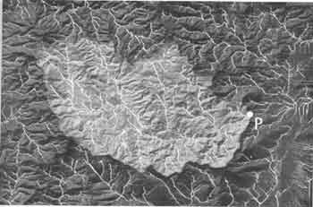
Figure 1 Shaded DEM Image with Drainage Pattern
MOS-1 MESSR data were used as remote sensing data which were received on 7 February 1989. It was cloud free data. The MOS-1 MESSR data should be corrected geometrically in order to overly DEM which coordinate system of DEM was UTM. A geometric correction was carried out by pseudo-affine transformation with GCPs. The corrected MOS-1 MESSR data were shown in Figure2.
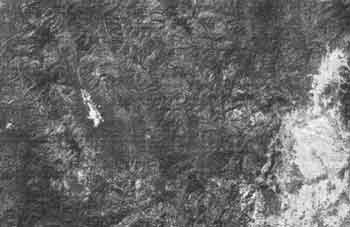
Figure 2 MOS-1 MESSR Image
As hydrologic data, precipitation and discharge data could be acquired. The hydrologic data were observed from 1987 to 1989. The observatory point was shown as point P on Figure 1.
Hydrologic Feature in Test Area
Hydrograph in 1987 was shown in Figure 3 . From this graph, a period of rainy season ranges from June to Novembe The runoff discharge depends upon precipitation normally. Though it is very sensitive in July and August, it is not so sensitive in May, June and November. The sensitivity depends upon precipitation intensity. An infiltration capacity is influenced by soil moisture which is changed by precipitation intensity . The infiltration capacity can be estimated by horton Equation or Philip Equation. On the other hand, the rujnoff discharge decrease smoothly after November . The discharge was supplied from base runoff discharge which means ground water. Usually, a base runoff discharge is supposed as constant value in runoff anal6sis. However, it should be set as variable value in this test area.
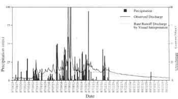
Figure 3 Observed Hydrograph in 1987
By the way, this observed hydrograph (Figure 3) has some strange results. For example, runoffdischarge increase suddenly in spite of no precipitation in the end of June. Reversely, runoff discharge doesn'' increase very much in spite of huge precipitation in the begiinning of October, The reason might come from huge catchment area and locally changeable eather. Perhaps, if heavy rain was observed at point "P" it might be no precipitation in other area. We must carried out runoff anysis in such situation even though there is not other helful climate data in this study.
Developed Model
Figure 4 Flow Chart of Runoff Analysis
In this study, a hydraulic model is based on a grid series tank model. Figure 4 shows flow chart of runoff analysis. Firstly, a precipitation is supplied to each DEM grid that is one of the tanks. The supplied precipitation shich means inlet content is calculated by following equation
Q in = K I R L 2
Qin: Inlet Content (m3)
Ki: Infiltration
R: Precipitation (m)
L: Grid Size (m)
In this equation, infiltration is usually depend upon landcover, Nakano (1) showed relationship between infiltration and landcover. In this study, we adopted his results, and the infiltration was led from NDVI which is calculated from MOS-1 MESSR data. The relationship between infiltration and NDVI is shown as follows'
| Bare Soil | Glassland | Forest | |||||
| NDVI : | -1.0 | ¨ | 0.1 | ¨ | 0.25 | ¨ | 1.0 |
| Infiltration (mm/h) | 30 | 100 | 270 |
Next, the inlet content divides into three discharges which are evapotranspiration, infiltration and surface flow. Moreover, the infiltrated we\ater was divided into three discharges which are sbsurface flow, base flow and dead water.
A decision of runoff percentage of surface flow and subsurface flow is very important. The runoff percentage is changed by season, which is influenced by precipitation intensity. Table 1 shows runoff percentage in each season, which were calculated from the hydrograph (Figure 3) The runoff percentage shows tendency to increase according to rainy wseason. In this study the runoff percentages can be set by proportional equation with calculated runoff percentage in dry season and rainy season. The surface runoff and the subsurface runoff in each tank can be expressed by following equations.
Q in = Kr Q in
Qin : Inlet Content (m3)
Kr: Runoff P rcentage
Q in : Effectiv Inlet (m3)
After that, the surface flow and the subsuface flow must be discharged to next grid according to slope aspect and velocity That is to say flow tracking. The slope aspect is calculated from DEM the velocity can be estimated from slope gradient which is also calculated from DEM. The surface flow and the subsurface flow in the grid can be experessed by a continuous equation as follows;
Q t+t = q in -q out)D t
Q : Remaining Countent (m2)
Qin: Inlet (m3/s)
Qout: Outlet (m3/s)
DT: Time (s)
By the way, an estimation of the base runoff is very difficult because the discharge includes ground water which is always supplied in spite of precipitation. In this study, the base runoff discharge was led from the observed hydrograph. A straight broken line in Figure 3 shows estimated base runoff discharge by using visual interpretation.
Table 1 Runoff Percentage in Each Season
| Dry Season Rainy | ® | Season | |
| Base Runoff | 13.84 | 7.53 | 9.36 |
| Subsurface Runoff | 1.95 | 3.01 | 6.92 |
| Surface Runoff | 2.13 | 4.22 | 14.12 |
| Total Runoff | 17.91 | 14.75 | 30.40 |
Results and Conclusions
By using previous model, estimation of total discharge was carried out. Figure 5 shows hydrograph in 1987 which are consist of estimated discharge, actual discharge and pecipitation. The result shows almost high accuracy. However, in the end of June and the beginning of October, etimated discharge was much different from actual one. The climate data and discharge data were observed at only one point. In monsoon area and mountainous area, climate is very changeable. Moreover, the cachment area in this study were too huge. It has been already mentioned in the previous chapter. So, it is impossible to represent climate data by only one observatory point. In future, bydrograph should be made from many climate data though we couldn't have enough observation points.
Figure 5 Estimated Hydrograph in 1987
In this study, estimation of runoff discharge was succeeded with use of remote sensing data, DEM and climate data. It will be used as time interpolation of runoff discharge. After all remote sensing data and DEM showed very helpful data for runoff analysis.
References
- Hideaki NAKANO, "Hydrology in Forest". Kyouritsu Shuppan, pp. 55-72 (in Japanese)
- Shiro OCHI, Shunji MURAI and Suvit VIBULSRESTH, " Flood Disaster Prediction Model using Remote Sensing Data and Geographic Information System", proceedings of the 10th ACRS, PP B-3-1-b-3-6
- Sahido SUSANTO and Yoshihiro KAIDA, "Tropical Hydrology Simulation Model for Watershed Management", Journal of Japan Society of Hydrology Simulation Model for Watershed Management Journal of Japan Society of Hydrology and Water Resource, Vol.4 No. 2, PP. 430-53