| GISdevelopment.net ---> AARS ---> ACRS 1994 ---> Disasters |
Flood Study in the Meghna -
Dhonagoda Polder, Bangladesh
J. A. M. de Brouder
International Institute for Aerospace Survey and Earth Sciences
The Netherlands
J. A. M. de Brouder
International Institute for Aerospace Survey and Earth Sciences
The Netherlands
Introduction
Geographic information systems and remote sensing (thereafter abbreviated to GIS and RS) provide a broad range of tools for determining areas affected by floods or for forecasting areas likely to be flooded due to high river or sea water levels. For an effective management of flood water in low lying flood-prone areas, GIS and RS technology is proving to be a useful and efficient instrument *Wagner, 1989, Wu, Bingfang et al., 1990 and Rahman, 1992).
Satellite images taken during or after the period of flooding provide an effective means of mapping the extent of the flooded areas. The frequent coverage b the satellites provides the most up-to-data relevant to the flooded area.
Spatial data stored in the digital data bas of the GIS, such as digital elevation model (DEM), can be used to predict the effects of future events. The extent of inundation and the depth of flooding can be forecasted. The GIS data base may also contain agricultural, socio-economic, communication, population and infrastructure data. This can be used, in conjunction with the flooding data. for an evacuation strategy, in conjunction with the flooding data, for and evacuation strategy, rehabilitation planning or damage assessment.
Bangladesh, situated in one of the world's highest precipitation areas, is accustomed to flooding due to its low topography with some of the world's biggest rivers flowing through it, and occurrence of cyclones.
The severe floods that strike Bangladesh regularly cause and immense loss of life and property and put a heavy burden on the economy of the country. The floods in 1987 and 1988 caused a total damage of US$ 500 million and US$ 1300 million respectively. In 1987 39% of the country was flooded, affecting 30 million people. Loss of the main crop (paddy) was estimated to be 0.8 million tones. For 1988 these figures were 60% of the country, 45 million people and 1.8 million tones of paddy. It is clear that damage to infrastructure (roads, bridges, railways, irrigation structures, etc.) and buildings (villages, schools, hospitals, etc) was also enormous (World Bank, 1989).
The Study Area
The study area (35km2) is part of a polder that lies in the middle Meghna floodplain, that occupies a small area at the confluence of the Gangas river and the Meghna river (Figure 1.1). It is a low-lying landscape of meander scrolls, natural levees, other ridges, backswamps and channels. The area has an elevation of 0.9 m to 3.66 m (SOB datum) above mean sea level.
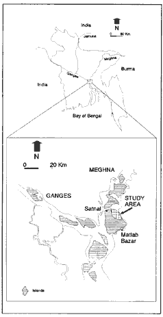
Figure 1.1 Location of the study area
The population dentist is high. According to the census in 1984 it was 1195 persons/sq.km.. Assuming an annual increase of 3.6%, at present there are more than 2000 persons per sq. km. This is particularly high for a rural area.
Most of the land is used for agriculture. Housing and horticulture (fruit trees and vegetables) are found on the higher ridges; paddy is grown in the lower-laying basins. In those places where the villages are located, the ridges have sometimes been heightened by man to reduce the effects of flooding.
The average yearly precipitation is 2500 mm of which 75% occurs during the monsoon from June to October. However, in the dry winter period from November to February, depressions in the Bay of Bengal may cause cyclones that carry substantial amounts of rainfall and lead to a significant amount of damage. The average yearly evaporation equals about 1000 mm.
The area is subject to tidal influences. During the rainy season the tidal range is low (average 25 cm). This may be up to 1.4 m during the dry season.
In early September 1998 a disastrous flood hit Bangladesh. On September the 3rd the water rose to 6 meters above mean sea level due to high discharge and tide. This in combination with heavy rainfall, caused collapse of the dike protecting the polder. Like many other areas in Bangladesh, the study area was flooded. Crops were destroyed, infrastructure demolished and lives lost.
Objectives
The main objective was to assess GIS and RS as tools for managing flood - prone areas is Bangladesh. The specific objectives were:
Material on the study area included:
No water levels were recorded within the study area. Satnal is the closest station at a distance of about 10.5 km from the centre of the study area; Matlab Bazar is about 24.5 km from the centre.
Use was made of system which has integrated software for GIS and remote sensing operations (Meijerink et al., 1988).
Figure 1.2 shows a flowchart depicting the different steps taken during the analysis.
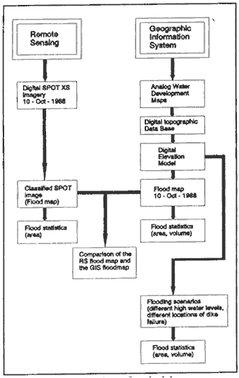
Figure 1.2 Flowchart of methodology
Creation of A Digital Elevation Model
A digital elevation model (DEM) is the numerical representation of the relief of (part of) the earth's surface. It represents a topographic surface in terms of a set of elevation values measured at a finite number of points and contains terrain features of morphologic importance such as valleys, ridges, peaks and pits. The GIS used creates and stores a DEM in raster format.
The DEM was created by digitizing the existing contour lines from topographic maps. The vector format with the contour lines was converted to raster format before interpolation took place. The selected cell size was 5 m. This ma seem excessively large but it was necessary in order to take into account the very steep slopes of the ridges the cross the area. The Bogefors distance transform was used to estimate the unknown elevation values for the locations between the isolines (Gorte, 1990). After the interpolation procedure the increase in the height of the ridges. In Bangladesh the houses are usually built on the ridges and in ordure to be safe from flooding an extra 1 to 1.5 m of soil is added to the ridges. The village boundaries were digitized and polygonized, and their elevation values on the DEM were increased by and arbitrary 1m.
Creation of Flood Maps
Creation of a flood map using the DEM
On October the 10th 1988 the low water level was about 3.00m a.m.s.l. and the high water level was about 3.50 m. The exact water level at the time of the image acquisition was not known.
Using the DEM, a map can be created showing the extent of the area that is inundated, provided that the DEM is accurate enough. By comparing this result flood map with the classified image an assessment of the quality of the DEM can be made (see Section 1.7).
If a dike fails at a certain location, inundation will occur in the areas in the polder that have an elevation lower that the outside water level and that are connected with the location of the dike failure. Simply slicing the DEM up to a certain flood level will not show the actual flooded area. In order to find the topographically connected areas a topographic operator (i.e., the neighborhood function ) of a GIS will have to be used in conjunction with a connectivity operator.
The flowchart in Figure 1.3 shows the interative process of obtaining the flooded area from a DEM.
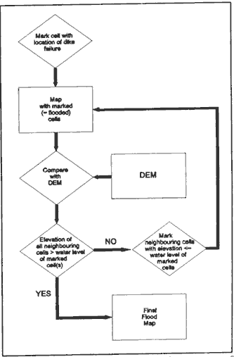
Figure 1.3 Flowchart showing the process of obtaining a flood map from a DEM
First a starting cell was created corresponding to the location of the dike failure. An algorithm sought all neighboring cells of the marked cell that have an elevation lower or equal to the specified flood level. These cells were also marked. The process continued comparing all neighboring cells of the newly marked cells with the flood level and again those cells with a lower or equal elevation compared to the flood level were selected. This procedure of iteration with propagation continued till no more cells were marked as flooded.
As the flood level on 10 October 1988 was between 3.00 and 3.50 m a.m.s.l. two flood maps were created: One for a water level of 3.00 m and one for a water level of 3.50m. The Figurers 1.4a and 1.4b show these flood maps resulting from the operation on the DEM. At a water level at 3.00 m 83% of the area was estimated to be flooded; at 3.50 m 90% of the area was found to be inundated.
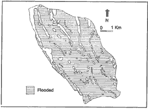
Figure 1.4a Estimated flooded area, using a DEM High water level of 3.00m

Figure 1.4b Estimated area flooded, using a DEM. Flood level of 3.50 m.
Creation of a flood map using SPOT multispectral imagery
Compare with the other landcover types, water bodies have a very low reflection in the near infrared bands and can be detected easily on digital remote sensing imagery. By using the simple technique of density slicing it was possible to differentiate between flooded and non-flooded areas. Figure 1.5 shows the flooded and non-flooded areas obtained by slicing the near infrared band image of 10 October 1988. It appeared that that 83% of the area was flooded.
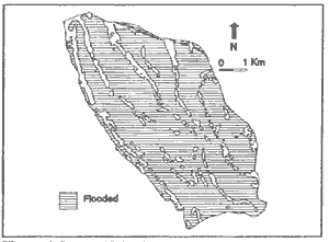
Figure 1.5 SPOT image classified as flooded and non-flooded areas, using density slicing.
For comparison, a multispectral classification was also performed. Five classes were sampled (vegetation, dike, housing, water bodies and clouds). Although there was some similarity between the spectral signature of the dike and the housing and between the vegetation and housing, this was not a problem as the interest laid in the distinction between water ad the non-flooded areas. In this case 81% of the area was classified as 'water bodies'. This compared well with the result of the density slicing.
Comparison with RS Imagery
In order to compare the flood maps obtained by processing of the SPOT imagery and the DEM, these two products have been overlayed and the differences and similarities were analyzed.
Figure 1.6 shows, as an example, the comparison of the flooded/non-flooded areas on the image and the DEM for a flood level of 3.00 m.
Figure 1.6 Comparison between flooded areas on image and DEM (flood level : 3.00 m)
Table 1.1 gives the statistics on the differences and similarities. From this table it appears that the percentages of flooded area and non-flooded area obtained by slicing the image and b using the DEM with a water level of 3.00 m are the same (83% and 17% respectively). The flood map derived from the DEM with a water level of 3.50 m gives higher percentage of flooded area. Although the differences were within an acceptable range, there are inconsistencies if one looks at the values of Table 1.2
For 86% (water level: 3.00m) and 88% (water level: 3.50 m) the results of the DEM operations matched the satellite image flood map. However, about 41% of the non-flooded area on the image was shown as flooded on the DEM (water level: 3.00m). For the water level of 3.50 m. value was 56%.
Table 1.1 Comparison of flooded and non-flooded areas on the image and DEM (assumed water levels of 3.00 and 3.50 m).
Table 1.2 Result of overlaying the flood map obtained from the image and the DEM (assumed water levels of 3.00 and 3.50m.)
Calculation of The Area, Depth and Volume of The Flood Waters
Once the flood maps had been created, the areas could be calculated. The number of flooded raster cells multiplied by the area of 1 cell gave the total flooded area.
For determining the depth of the flood water the DEM was uses. Subtracting the elevation value for each flooded cell from a specified flood level gave the flood depth. The resultant map could be classified to show the deeply, moderately and shallowly flooded lands. Figure 1.7 shows the flood depth map of the flood with a flood level of 3.00 m.
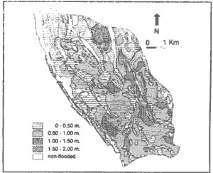
Figure 1.7 Flood depth map (flood level : 3.00 m)
If an area is flooded and the water has to be evacuated, either by pumping or gravity, it is important to know the flood water volume. This volume determines the pump or the spill capacity if it is necessary to drain the water within a limited time period, required to avoid more damage to the standing crop or because a new crop has to be planted for the next season. Having a flood depth map the volume can be calculated by multiplying the area of each cell with the corresponding depth value and then aggregating these volumes per cell for the tow flood levels.
The Effects on Depth, Area and Volume of The Flood Waters Given Different Flooding Scenarios
For the management of flood-prone areas it is important to assess the expected consequences of possible flooding events. The effects of different storm water
Table 1.3 Flood statistics for a flood level of 3.00 m and 3.50 m.
levels are of interest, as well as the effects of a dike failure at different locations. Does dike failure have the same consequences wherever it my occur or would its occurrence at one point lead to more severe damage than its occurrence at another point? In other words, does it matter where the dike collapses?
For five different locations the effects of flooding in terms of depth, aea and volume were evaluated for different storm water levels. Figure 1.8 shows the assumed locations of the dike failure. Location 1 is the actual location of the dike failure on 10 October 1988.

Figure 1.8 Assumed locations of a dike failure.
Table 1.4 shows the results of the analysis. It reveals that below a storm water level of 3.75 m it does matter where the dike fails. Above this water level all five situations leas to the same effect.
Table 1.4 Volume of flood waters for 5 assumed locations of dike failure
References
Geographic information systems and remote sensing (thereafter abbreviated to GIS and RS) provide a broad range of tools for determining areas affected by floods or for forecasting areas likely to be flooded due to high river or sea water levels. For an effective management of flood water in low lying flood-prone areas, GIS and RS technology is proving to be a useful and efficient instrument *Wagner, 1989, Wu, Bingfang et al., 1990 and Rahman, 1992).
Satellite images taken during or after the period of flooding provide an effective means of mapping the extent of the flooded areas. The frequent coverage b the satellites provides the most up-to-data relevant to the flooded area.
Spatial data stored in the digital data bas of the GIS, such as digital elevation model (DEM), can be used to predict the effects of future events. The extent of inundation and the depth of flooding can be forecasted. The GIS data base may also contain agricultural, socio-economic, communication, population and infrastructure data. This can be used, in conjunction with the flooding data. for an evacuation strategy, in conjunction with the flooding data, for and evacuation strategy, rehabilitation planning or damage assessment.
Bangladesh, situated in one of the world's highest precipitation areas, is accustomed to flooding due to its low topography with some of the world's biggest rivers flowing through it, and occurrence of cyclones.
The severe floods that strike Bangladesh regularly cause and immense loss of life and property and put a heavy burden on the economy of the country. The floods in 1987 and 1988 caused a total damage of US$ 500 million and US$ 1300 million respectively. In 1987 39% of the country was flooded, affecting 30 million people. Loss of the main crop (paddy) was estimated to be 0.8 million tones. For 1988 these figures were 60% of the country, 45 million people and 1.8 million tones of paddy. It is clear that damage to infrastructure (roads, bridges, railways, irrigation structures, etc.) and buildings (villages, schools, hospitals, etc) was also enormous (World Bank, 1989).
The Study Area
The study area (35km2) is part of a polder that lies in the middle Meghna floodplain, that occupies a small area at the confluence of the Gangas river and the Meghna river (Figure 1.1). It is a low-lying landscape of meander scrolls, natural levees, other ridges, backswamps and channels. The area has an elevation of 0.9 m to 3.66 m (SOB datum) above mean sea level.
Figure 1.1 Location of the study area
The population dentist is high. According to the census in 1984 it was 1195 persons/sq.km.. Assuming an annual increase of 3.6%, at present there are more than 2000 persons per sq. km. This is particularly high for a rural area.
Most of the land is used for agriculture. Housing and horticulture (fruit trees and vegetables) are found on the higher ridges; paddy is grown in the lower-laying basins. In those places where the villages are located, the ridges have sometimes been heightened by man to reduce the effects of flooding.
The average yearly precipitation is 2500 mm of which 75% occurs during the monsoon from June to October. However, in the dry winter period from November to February, depressions in the Bay of Bengal may cause cyclones that carry substantial amounts of rainfall and lead to a significant amount of damage. The average yearly evaporation equals about 1000 mm.
The area is subject to tidal influences. During the rainy season the tidal range is low (average 25 cm). This may be up to 1.4 m during the dry season.
In early September 1998 a disastrous flood hit Bangladesh. On September the 3rd the water rose to 6 meters above mean sea level due to high discharge and tide. This in combination with heavy rainfall, caused collapse of the dike protecting the polder. Like many other areas in Bangladesh, the study area was flooded. Crops were destroyed, infrastructure demolished and lives lost.
Objectives
The main objective was to assess GIS and RS as tools for managing flood - prone areas is Bangladesh. The specific objectives were:
- To create a DEM of the study area.
- To create a flood map of the study area using the digital elevation
model assuming the same high water level as during in 1988.
- To create a flood map of the study area for the 1999 flood using
SPOT multi spectral imagery.
- To compare the 1988 flood maps of the study area obtained by
satellite imagery and the DEM.
- To calculate the acreage of the area flooded and the depth and
volume of the flood waters for the study area for the 1988 flood.
- To assess the effect of flooding (area extent, depth and volume)
assuming different high water levels and different locations of dike
failure.
Material on the study area included:
- SPOT Multispectral CCT of 10 October 1988,
- Water Development Maps 1:15840 (Survey of Bangladesh, 1978).
- Daily high and low tide water levels from Satnal for 1988.
- Daily high and low tide water level from Matlab Bazar for
1988.
No water levels were recorded within the study area. Satnal is the closest station at a distance of about 10.5 km from the centre of the study area; Matlab Bazar is about 24.5 km from the centre.
Use was made of system which has integrated software for GIS and remote sensing operations (Meijerink et al., 1988).
Figure 1.2 shows a flowchart depicting the different steps taken during the analysis.
Figure 1.2 Flowchart of methodology
Creation of A Digital Elevation Model
A digital elevation model (DEM) is the numerical representation of the relief of (part of) the earth's surface. It represents a topographic surface in terms of a set of elevation values measured at a finite number of points and contains terrain features of morphologic importance such as valleys, ridges, peaks and pits. The GIS used creates and stores a DEM in raster format.
The DEM was created by digitizing the existing contour lines from topographic maps. The vector format with the contour lines was converted to raster format before interpolation took place. The selected cell size was 5 m. This ma seem excessively large but it was necessary in order to take into account the very steep slopes of the ridges the cross the area. The Bogefors distance transform was used to estimate the unknown elevation values for the locations between the isolines (Gorte, 1990). After the interpolation procedure the increase in the height of the ridges. In Bangladesh the houses are usually built on the ridges and in ordure to be safe from flooding an extra 1 to 1.5 m of soil is added to the ridges. The village boundaries were digitized and polygonized, and their elevation values on the DEM were increased by and arbitrary 1m.
Creation of Flood Maps
Creation of a flood map using the DEM
On October the 10th 1988 the low water level was about 3.00m a.m.s.l. and the high water level was about 3.50 m. The exact water level at the time of the image acquisition was not known.
Using the DEM, a map can be created showing the extent of the area that is inundated, provided that the DEM is accurate enough. By comparing this result flood map with the classified image an assessment of the quality of the DEM can be made (see Section 1.7).
If a dike fails at a certain location, inundation will occur in the areas in the polder that have an elevation lower that the outside water level and that are connected with the location of the dike failure. Simply slicing the DEM up to a certain flood level will not show the actual flooded area. In order to find the topographically connected areas a topographic operator (i.e., the neighborhood function ) of a GIS will have to be used in conjunction with a connectivity operator.
The flowchart in Figure 1.3 shows the interative process of obtaining the flooded area from a DEM.
Figure 1.3 Flowchart showing the process of obtaining a flood map from a DEM
First a starting cell was created corresponding to the location of the dike failure. An algorithm sought all neighboring cells of the marked cell that have an elevation lower or equal to the specified flood level. These cells were also marked. The process continued comparing all neighboring cells of the newly marked cells with the flood level and again those cells with a lower or equal elevation compared to the flood level were selected. This procedure of iteration with propagation continued till no more cells were marked as flooded.
As the flood level on 10 October 1988 was between 3.00 and 3.50 m a.m.s.l. two flood maps were created: One for a water level of 3.00 m and one for a water level of 3.50m. The Figurers 1.4a and 1.4b show these flood maps resulting from the operation on the DEM. At a water level at 3.00 m 83% of the area was estimated to be flooded; at 3.50 m 90% of the area was found to be inundated.
Figure 1.4a Estimated flooded area, using a DEM High water level of 3.00m
Figure 1.4b Estimated area flooded, using a DEM. Flood level of 3.50 m.
Creation of a flood map using SPOT multispectral imagery
Compare with the other landcover types, water bodies have a very low reflection in the near infrared bands and can be detected easily on digital remote sensing imagery. By using the simple technique of density slicing it was possible to differentiate between flooded and non-flooded areas. Figure 1.5 shows the flooded and non-flooded areas obtained by slicing the near infrared band image of 10 October 1988. It appeared that that 83% of the area was flooded.
Figure 1.5 SPOT image classified as flooded and non-flooded areas, using density slicing.
For comparison, a multispectral classification was also performed. Five classes were sampled (vegetation, dike, housing, water bodies and clouds). Although there was some similarity between the spectral signature of the dike and the housing and between the vegetation and housing, this was not a problem as the interest laid in the distinction between water ad the non-flooded areas. In this case 81% of the area was classified as 'water bodies'. This compared well with the result of the density slicing.
Comparison with RS Imagery
In order to compare the flood maps obtained by processing of the SPOT imagery and the DEM, these two products have been overlayed and the differences and similarities were analyzed.
Figure 1.6 shows, as an example, the comparison of the flooded/non-flooded areas on the image and the DEM for a flood level of 3.00 m.
Figure 1.6 Comparison between flooded areas on image and DEM (flood level : 3.00 m)
Table 1.1 gives the statistics on the differences and similarities. From this table it appears that the percentages of flooded area and non-flooded area obtained by slicing the image and b using the DEM with a water level of 3.00 m are the same (83% and 17% respectively). The flood map derived from the DEM with a water level of 3.50 m gives higher percentage of flooded area. Although the differences were within an acceptable range, there are inconsistencies if one looks at the values of Table 1.2
For 86% (water level: 3.00m) and 88% (water level: 3.50 m) the results of the DEM operations matched the satellite image flood map. However, about 41% of the non-flooded area on the image was shown as flooded on the DEM (water level: 3.00m). For the water level of 3.50 m. value was 56%.
Table 1.1 Comparison of flooded and non-flooded areas on the image and DEM (assumed water levels of 3.00 and 3.50 m).
| Image | Water level: 3.00m | Water level: 3.50 m | |
| Flooded | 83 | 83 | 90 |
| Non-flooded | 17 | 17 | 10 |
Table 1.2 Result of overlaying the flood map obtained from the image and the DEM (assumed water levels of 3.00 and 3.50m.)
| Water level 3.00 m | Water level 3.50 m | ||
| Index | % | Index | % |
| 1 | 10 | 1 | 7 |
| 2 | 7 | 2 | 9 |
| 3 | 7 | 3 | 3 |
| 4 | 76 | 4 | 81 |
key to index:A number of reasons may account for the differences in the results of the different methods. Some soils might have been very moist and had the same reflection as shallow water; the flood level at the time of the acquisition of the image was not known, and/or the assumption that the water surface was level might not have been valid. Probably the most important reason was the quality of the DEM. Firstly the map was 20 years old and as the population in the area had doubled in the meantime, the development of houses along the ridges mould have influenced the topography. Secondly the contours on the map were constructed by interpolating between the points of a grid for which the elevation was measured. The survey was done along lines, and used more or less equal distances between points. The detailed geomorphology was not considered. Consequently the DEM was more inaccurate along the ridges. Thirdly, the addition of 1 m of extra height to the ridges might not have been appropriate in all cases.
1 Non-flooded on both image and DFM
2 Flooded on DEM, non-flooded on image
3 Non-flooded on DEM, flooded on image
4 Flooded on both image and DEM
Calculation of The Area, Depth and Volume of The Flood Waters
Once the flood maps had been created, the areas could be calculated. The number of flooded raster cells multiplied by the area of 1 cell gave the total flooded area.
For determining the depth of the flood water the DEM was uses. Subtracting the elevation value for each flooded cell from a specified flood level gave the flood depth. The resultant map could be classified to show the deeply, moderately and shallowly flooded lands. Figure 1.7 shows the flood depth map of the flood with a flood level of 3.00 m.
Figure 1.7 Flood depth map (flood level : 3.00 m)
If an area is flooded and the water has to be evacuated, either by pumping or gravity, it is important to know the flood water volume. This volume determines the pump or the spill capacity if it is necessary to drain the water within a limited time period, required to avoid more damage to the standing crop or because a new crop has to be planted for the next season. Having a flood depth map the volume can be calculated by multiplying the area of each cell with the corresponding depth value and then aggregating these volumes per cell for the tow flood levels.
The Effects on Depth, Area and Volume of The Flood Waters Given Different Flooding Scenarios
For the management of flood-prone areas it is important to assess the expected consequences of possible flooding events. The effects of different storm water
Table 1.3 Flood statistics for a flood level of 3.00 m and 3.50 m.
| Flood level (m) | Area Flooded (million ha) | Volume of flood waters (million m3) |
| 3.00 | 2.89 | 1634799 |
| 3.50 | 3.16 | 2443454 |
levels are of interest, as well as the effects of a dike failure at different locations. Does dike failure have the same consequences wherever it my occur or would its occurrence at one point lead to more severe damage than its occurrence at another point? In other words, does it matter where the dike collapses?
For five different locations the effects of flooding in terms of depth, aea and volume were evaluated for different storm water levels. Figure 1.8 shows the assumed locations of the dike failure. Location 1 is the actual location of the dike failure on 10 October 1988.
Figure 1.8 Assumed locations of a dike failure.
Table 1.4 shows the results of the analysis. It reveals that below a storm water level of 3.75 m it does matter where the dike fails. Above this water level all five situations leas to the same effect.
Table 1.4 Volume of flood waters for 5 assumed locations of dike failure
| Flood level (m2) | Volume of flood waters (million m3) | ||||
| Locations | |||||
| 1 | 2 | 3 | 4 | 5 | |
| 200 | 0 | 0 | 0 | 0 | 0 |
| 225 | 0.38 | 0 | 0 | 0 | 0 |
| 250 | 5.73 | 0 | 5.73 | 0 | 0 |
| 275 | 11.06 | 0 | 11.06 | 11.06 | 0 |
| 300 | 17.94 | 17.94 | 17.94 | 17.94 | 0 |
| 325 | 25,55 | 25.55 | 25.55 | 25.55 | 0 |
| 350 | 33.39 | 33.39 | 33.39 | 33.39 | 0 |
| 375 | 41.35 | 41.35 | 41.35 | 41.35 | 41.35 |
References
- Gorte, B. et, 1990. Interpolation between insolines based on the
Bagefors distance transform. ITC Journal 1990-3, ITC, Enschede, The
Netherlands.
- Meijerink, A.M.J., C.R. Valenzuela & A. Stewart (eds.) 1988.
ILWIS, the Intergrated Land and Watershed Management Information System.
ITC Publication No 7, Enschede, The Netherlands.
- Rahman, A.K.M., 1992. Use of FIS, Remote Sensing and Models for
flood studies in Bangladesh. An analytical study in a flood prone polder
in Bangladesh. Unpublished MSc Thesis, ITC. 94P.
- Survey of Bangladesh. 1978. Water Development Maps 1:15,840, No 79
(I-11) and 79 (I-11)/7
- Wagner, Th. W., 1989. Preparing for floodplain mapping and flood
monitoring with Remote Sensing and GIS. Report of the workshop on remote
sensing for floodplain mapping and flood monitoring, Dhka,
Bangladesh.
- Worldbank, 1989. Bangladesh Action Plan for Flood Control.
- Wu, Bingfang & Xia, Fuxiang, 1990. Flood damage evaluation
system design for a pilot area on Bangladesh floodplain fusing remote
sensing and GIS. European Conference and
GIS.