GISdevelopment.net ---> AARS ---> ACRS 1992 ---> Digital Image Processing Neural network structure generation for the classification of remotely sensed data using simulated annealing Hosomura, P.K.M.M. Pallewatta, H.N.D. Karunasekara Division of Computer Science Asian Institute of Technology GPO Box 2754, Bangkok 10501, Thailand Abstract Artificial feed forward neural networks are increasingly being used for the classification of remotely sensed data. however the back propagation algorithm, which is so widely used does not provide any information about the structure of the network for a given classification problem. Minimum sizes networks are important for efficient classification and good generalization. This paper describes a method to simultaneously learn the structure and the weights of the networks from training data using Simulated Annealing optimization technique. Introduction The use of artificial neural networks (ANNs) as classifiers as an alternative to statistical classification has become popular since the development of the back propagation algorithm. Feed forward ANNs, trained by back propagation have been used by several researchers for the classification of remotely sensed data. Please refer to (4) and (5) for details about back propagation. One of the most common difficulties encountered by all the researchers is that the structure of the networks, that is optimal for a given classification task is unknown. Often researchers select the structure by starting from a minimal seized network and increase the nodes in the hidden layers until the network can be successfully trained. Alternatively they may get a rough idea about the structure by observing the data (training data in a Remote Sensing context) in feature space. Back propagation does not provide us with any idea about the structure of the network for a given classification problem and it does not guarantee a solution. A network too small for a given problem will cause back propagation not to coverage to a solution while larger ones lead to poor generalization. Large networks also consume more resources while smaller ones can be efficient in software implementations. The technique proposed here simultaneously learns the weights and the minimal structure for a given classification problem by minimizing a cost function that is proportional to the total error over the pattern set, to the number of nodes and to the number of connections in the network. Simulated annealing is being employed as a technique to perform the optimization due to it's ability to optimize very complex problems. Our approach is slow due to the use of simulated annealing, which can be considered as a disadvantages. Simulated Annealing This technique was introduced in 1983 by Kirkpatrick et al as a tool to solve complex optimization problems. In physical systems the state of minimum energy is called the ground state. Simulated annealing treats the system to be optimized as a physical system and function to be minimized as an energy function. Then the problem of combinatorial optimization transforms to a problem of finding the ground states of the system. With simulated annealing, one starts at a very high temperature and simulates the slow cooling process of a physical system, reducing the temperature slowly to reach the ground state. The cooling must be slow enough so that the system does not get stuck in metastable states that are local minima of the energy. 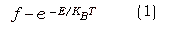For a given temperature states of a physical system is described by the distribution, E - energy of the state kB - Boltzmann's constant T - absolute temperature It should be noted that the concept temperature in physical systems have no Obvious equivalent in optimization problems. In simulated annealing temperature will be a parameter that controls the randomness of the states accepted. 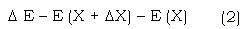The algorithm for simulated annealing is as follows. Let X be a vector of variables and E(X) be the function to be minimized. The temperature is kept at a high value initially. One starts with a random value of X and a small random perturbation DX attempted. The energy change in the system caused by this DE caused by this perturbation is computed. If the perturbation has reduced the energy function (i.e DE < 0), it is accepted and the new state X + D E > 0 the perturbation is accepted with a probability of e-DE/T. The sequence of states produced by this algorithm is distributed according to (1) [2]. At high temperatures the e-DE/T is close to 1 regardless of DE. So almost all perturbations are accepted and the resulting configurations (States) area very random. But at low temperatures this expression for the probability of acceptance favors perturbations that tend to keep the energy low. The initial heating up of the system is necessary to make the final state independent of the initial state (3). In cooling the system, one should slowly reduce the temperature only after thermodynamic equilibrium has been reached at the current temperature and the procedures should continue until T = 0. In practice there are many cases, where there are many minima very close to the absolute minimum. In such case it will be sufficient to find one of them [2]. For problems of constrained minimum, the method can be adapted by excluding the perturbations that do not satisfy the constraints [1] [2]. Simulated annealing can also be applied to discrete optimization [1]. For a more detailed description of simulated annealing please refer to [1]. Neural Network Structure Generation Supposing we are given a set of training data samples along with their respective classes. If the input data are n dimensional real vectors and the classes are m dimensional real vectors, the mapping that exists between them is a function f : R > Rm . Our task is to find a network N', which computers this function. 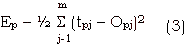If we are given a function f : R - > Rm, the error produced by this network for pattern pair (training data + class vectors) can be expressed as in [4], tpj - Target value of the jth position of pattern p. Opj- output value of N' the jth position for pattern p. and the total error accumulated over the training set can be expressed as, np - num of patterns. Our object would be to minimize E, so that N' approaches N. Before we discuss minimization with simulated annealing, some points have to be made clear. According to Kolmogorov's theorem [5], any decision region (possibly non convex and discontinuous) can be formed by a network with two hidden layers. So we will limit our networks to a maximum of two hidden layers. 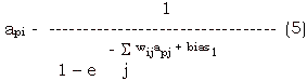It is better if the non linearities associated with neurons to be differentiable. This will allow us to identify whether every perturbation made to the system is energetically favorable or not. This can help in speeding up the search. Sigmoid non-linearities described in (5) can be used here. With sigmoid non-linearities the input-output relationship of a mode can be stated as follows. where api, apj - activation of nodes i and j for pattern p. biasi - bias node i wij - weight of connection from node to node i. The following events can be used as perturbations to the system. adding a node adding of connection removing of a node weight change of connection The following constrains may be observed to improve the effectiveness of the algorithm. The generation of the above mentioned events can be weighted by probability factors. As an example, weight change or bias change may be more probable that adding a neuron. If a node's input or output connections are fully removed then that node may be removed from the network. Since the dimensionally of input and output patterns are fixed the number of nodes in the input and output layers are fixed. The annealing can start from a random configuration of the network and the system will be heated up from than point and allowed to cool down. 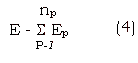Minimizing the expression eq. (4) is of no use because it does not tend to limit the degrees of freedom. Bu taking a large network the error over the training pattern set may be minimized, but such a solution is of hardly any use for the following reasons. Such large networks lack generalization. Generalization is the ability of the network to respond correctly to patterns which were not presented during training. This is the most important point on which neural networks differ from lookup tables. Large networks are computationally expensive. This will increase hardware costs if implemented in hardware adversely affect the efficiency if implemented in software. To overcome the above mentioned problems, we have to penalize solutions with large number of nodes and connections. This can be done by formulating the objective functions as follows Where a - penalizing constant for nodes Nn - num. of nodes in network b - penalizing constant for connections Nc - num of connections in network. E - total error over pattern set as in eq. (4) The role of constants a and b can be explained as follows. If we increase these constants the contribution to error due to nodes and connections increase respectively. This will cause the system to favor solutions with less nodes and connections respectively. Operational scheme for classification In an Operational scheme for classification, training data from the image to be classified can be fed to a system based on the above mentioned principles and the system's output will be an ANN to perform the classification along with the weights and the biases of the network. Then this network can be implemented on a programmable neural network card or by using software to perform the actual classification. Expected Results It is expected that using the objective function eq. (7), it will be possible to find neural network structures for the efficient classification of remotely sensed data. The networks are also expected to have good generalization capabilities. However the annealing schedules must be carefully designed equilibrium must be reached at each temperature as it was stated before. At present programs are being developed to carry out the simulation. This research is being carried out using MOS-1 MESSR data. The authors expect to present the results at the 13th ACRS in October 1992. References S. Kirkpatrick, C. Gelatt, and M. Vecchi, Optimization by simulated annealing, Science 220, 1983. P. Carvevali, S. Coletti and S. Patarnello, Image processing by simulated annealing. IBM Journal of Research and Development, Vol. 29, No. 6, November 1985 Donald E. Brown and Christopher L. Huntley, A practical application of simulated annealing, Pattern Recognition, Vol. 25, No. 4, 1992. J.L. McClelland D.E. Rumelhart, Parallel distributed processing, explorations in microstructure of cognition, Vol. 1, MIT Press, Cambridge, MA, 1986. R.L. Lippman, an Introduction to computing using neural nets, IEEE ASSP magazine, No. 4. Acknowledgement The authors wish to thank NASDA Bangkok office and the Nationals Research Council of Thailand for providing the raw data for this research.