| GISdevelopment.net ---> AARS ---> ACRS 1991 ---> Poster Session |
Digital Image Mosaicing
R. Parvathi, V
Jayaraman
Earth Observation System Indian Space Research Organisation
Bangalore-560094
S. Kannan
Regional Remote Sensing Service Centre
Earth Observation System Indian Space Research Organisation
Bangalore-560094
S. Kannan
Regional Remote Sensing Service Centre
Introduction
A problem which frequently arises when two or more scenes are mosaiced is the creation of artificial edges at the seams between the images. These artificial edges occur where there are perceptible radiometric differences within the region of overlap. The radiometric differences between images are usually caused by changes in atmospheric and earth surface conditions. Changes in atmospheric transmittance will tend to transform the grey scale over the whole image. Illumination caused by different sun angle, changes caused by human activities, precipitation and seasonal changes of surface multitemporal images. All these factors make it difficult for manual or photographic methods to produce image mosaics without artificial edge.
The Remote Sensing images may be mosaiced to a map projection or a reference image. Inaccuracy and uncertainty in determination of data on spacecraft and position, orientation and dam era attitude data cause registration error. Thus the image should be geometrically corrected and registered prior to mosaicing. The image mosaic process consists of four steps, namely (i) geometric registration of the input images. (ii) a grey level adjustment for each image in order to match their grey level histograms in the overlap region (iii) a seam point identification, at which the corresponding lines in the two images will be jointed, (iv) averaging the degree of mismatch of the grey level in the overlap region over the neighbourhood of the seam point.
Geometric correction is carried out using higher order polynomial transformation model. Linear Histogram Analysis Operation (LHAO) is used to perform radiometric temporal scene normalization. A two dimensional seam point searching algorithm (Yang Shiren et al, 1989) is implemented to select the best seam points. Through nearest neighbourhood interpolation the degree of mismatch of the grey level in the overlap region is averaged over the neighbourhood of the seam point.
Grey – Level Normalisation
If A, B be are the images which are being mosaiced and WA & WB are their respective overlapping windows, ideally, WA and WB are identifical (radiometrically), but in general they will not be identical due to various resons including atmospheric and surface conditions. Atmospheric and sensor conditions tend to operate on the grey level distribution rather than on spatial features and it is appropriate to ask what grey level mapping should be applied to minimize these changes. More specifically, if HWA, HWB are the histrograms of WA, WB respectively. A and B are transformed (requantized) so that HWAºHWB.
In contrast to atmospheric and sensor effects, the ground changes, produce grey level differences that are irreconcilable by histogram remapping. Therefore to define the appropriate grey level transformation one should exclude the regions that occur in only one of the overlapped images. Another case is where the grey level difference occurs due to ground reflectance changes. By masking the pockets where the changes occur the histogram should be calculated using rest of the image points (Milgram, 1975).
The radiation propagation to a Remote Sensing system may be modeled as: L = a * R + b where, L is the radiance reaching the sensor, R Reflectance of the target a is a factor including the solar irradiance, atmospheric transmittance and b is the radiation contribution by the air column.
Each term in the above equation is dependent on the spectral bandwidth and the solar geometry. In terms of temporal imagery, and define the characteristic changes in the illumination and atmospheric conditions, while R defines the characteristic feature changes and L is directly related to the brightness of the features in the image. Given two temporal images, the brightness values of feature within each image are modeled as :

The approaches to temporal image normalization to date involve the independent normalization of the individual images for the time varying effects. These techniques essentially normalize each image by correcting for the specific atmospheric and illuminating conditions on the specific date. The approach is to determine the scene specific values of ai and b to perform an independent conversion of each image to values representing surface reflectances, Ri. Studies have shown that the normalization techniques are generally only successful under optimal conditions and are not easily implemented due to the dependence on ground truth and/or characterization of the atmospheric conditions at the time of imaging. Because of these reasons, a simpler and effective approache is established to determine the transformation parameters is established to determine the transformation parameters (a1, a2, b1 and b2)using brightness distribution from each temporal image.
The method used to derive the normalization transforms in this study is a Linear Histogram Analysis Operation (LHA0). This method assumes that the transformation function is a linear transform and acts to align the central tendency and dispersion at the test distribution with that of the target distribution. Hence, given test distribution with the mean m2 and standard deviation s2, and a target distribution with mean m1, and standard deviation, 01, a linear transform, T, is defined as,

If the digital count values are linearly related to radiance, above transformation coefficients are used to define a linear combination of the input values which is applied locally by the equation Y (i, j) = a * X (i, j) + b
1 Seam Definition
Seam point searching is the process of selecting points in the overlap region which defines where one image ends and the other image begins. To define a vertical seam between two images it is necessary to select one point per line of overlap region. The image information to the left of the point will come from the line segment of the left hand side image and the information to the right from the right hand side image.
The seam point is chosen to produce the least amount of artificial edge. The edge that is proposed to be eliminated is not a physical edge but an edge corresponding to the grey value difference between the two overlapping regions. If the pixel grey values of the two images are f and g and their overlap region is N pixels wide, then the pixel values of the absolute grey difference image in the jth row are give by

If and edge measure computes 1 the sume of d j, k over u+1 pixels along jth row, to find the index value of k where

j=r, the seam would be at point k in row r.
This method finds a succession of points whose horizontal positions are unrelated. Such random positioning of the seam point reduces the visual edge. However, it has the disadvantage of introducing discontinuities in vertical direction. For example, if two successive seam points are in positions 10 and 20 respectively, then the image points in position 11 to 19 in the first line will come from the left hand side image, while those in the same positions in the next line will come from the right hand side image. If the left hand image differs significantly from the right one in this region a horizontal artificial edge will be seen.
An improvement of the one dimensional point selection method the two dimensional seam point search method (Yang Shirin et al 1989) has proved useful in avoiding horizontal artificial edge.
Let Vk and Hj be the vertical and horizontal edge measures, respectively; i.e.,
If the seam point in row r is (r, s), first search the seam point in row (r+1) to the right. Let

be the minimum vertical edge measure of points (r+1,s), (r+1, s+1), ……, (r+1, s+t) in the row r+1 for t = 0, 1, 2, ………., N-s-u/2, where N is the number of pixels in the row direction of the absolute-grey-difference image, and let

be the maximum horizontal edge measure of points ( r+1, s), (r+1, s+1), ….. , (r+1 s+t) in row r+1 for t = 0, 1, 2, … , N-s-u/2. The search on the right hand side beings from t=0, and is continued for t = 1, 2, 3, …. , N-s-u/2, if the difference between VR, t and HR, t on a per pixel bases, is less then or equal to a predefined threshold value,
Otherwise, the search on the right-hand side stops and starts the search on the left-hand side. In order to limit the artificial edges in the seams, the is selected in the range of L/32 to L/64, where L is the grey level dynamic range of the adjusted images. Similarly, let
be the minimum vertical edge measure and maximum horizontal edge measure of points (r+1, s-1), (r+1, s-2), …………….. , (r+1, s-t) in the row
After finishing the searches on the left-hand and right-hand sides, a best seam point in row 1+1 is selected by the formula Vr+1, s’ = MIN (VR, t’ VL, t). The best seam point in row r+1 is thus the point (r+1, s).
This two dimensional search restricts the range of seam points depending on the magnitude of the minimum edge difference (Dmin) on the previous line. Thus if the previous seam point had a large Dmin, the current seam point has to be chosen near the previous one.
In mosaicing of multispectral image data, if the seam points are searched on each component separately, the location of seam points will not coincide and artificial edge may appear in the red, green and blue components of the colour composite. In order to minimize the edges in a colour composite image, seam points are searched on the image pixel values which are the weighted sum of absolute – grey – difference. The abrupt grey level shift occurring in the neighbourhood of the seam point techniques.
Results and Discussions
After correcting the two IRS LISS IT A2, B2 images over Delhi for geometric distortions, the common portion of the overlap area is examined for brightness differences. LISS II A2 scene of Delhi is chosen to be the reference image for the mosaic and the radiometry of B2 scene of Delhi is transformed to achieve the best possible brightness match with A2 scene using Linear Histogram Analysis Operation. Figure 1 is the histogram of LISS II A2 scene of Delhi (29-47) Figure 2 is the histogram plot of the LISS II B2 scene of Delhi before and after grey level transformation using LHAO. Two dimensional seam point search algorithm is applied to the image of the weighted sum of absolute grey difference of three bands and the resultant image is shown in figure-3.
Fig 1: Histogram of LISS-II A2 Image of Delhi(29-47)
The SPOT multispectral images with path-row numbers of 215-324 and 216-324 are also mosiced using two dimensional seam point search algorithm. Figure 4 is the simple mosaic with straight seam points. It has apparent colour differences in the artificial edges in the image mosaic. The algorithm is applied on the mosaic SPOT images has no discernible edge and is shown in the figure 5.
Fig 2: Histogram of LISS-II B2 Image of Delhi
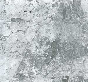
Fig 3: The Mosaic of IRS LISS II A2 B2 Image of Delhi with a Two dimensional seam point search on the image of weighted sum of absolute grey difference of three components
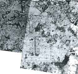
Fig 4: A MOSAIC of SPOT images with path-row numbers of 215-324 and 216-324 with stright seams
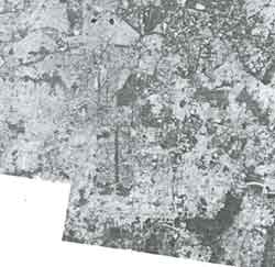
Fig 5: The MOSAIC with a two dimensional seam-point search on the images of weighted sum of absolute grey difference of three components
A two dimensional seam-point search algorithm with linear histogram analysis operation significantly eliminates the artificial edge in the image mosaic. However, the quality of the mosaic is strongly dependent on the quality of the input scenes. The better the scenes are matched in brightness and registered to each other, the better the final product. Thus, the availability of appropriate data can severely limit the quality of the final mosaic.
References
- Milgram D.L., 1975. Computer methods for creating photomosaics. Trans IEEE on Computers, Vol. C-24, pp 1113-1119.
- Milgram D.L., 1977. Adaptive techniques for photomosaicing. Trans. IEEE on Computers, Vol. C-26, pp 1175-1186.
- Susanne Hummer – Miller. , 1989. A Digital Mosaicing Algorithm allowing for an irregular joint ‘Line’. Photo Engg. and R. Sensing Vol. 55, No. 1, Jan. 1989, pp 43-47.
- Yang Shiren et al., 1989. Two dimensional Seam-point searching in Digital Image Mosaicing. Photo. Engg. And R. Sensing, Vol. 55, No. 1, Jan. 1989, pp 49-53.
- Peleg S., 1981. Elimination of Seam for Photomosaics. IEEE Conference on Pattern Recognition and Image Processing, pp 426-429.