| GISdevelopment.net ---> AARS ---> ACRS 1980 ---> Technical Session |
Unsupervised classification
of land sat MSS data
Y.J. Chong, A.C. Yeo, V.K,.
Vong and B.C. Chew
National University of Singapore
Singapore 1025
National University of Singapore
Singapore 1025
The Landsat scene covering Singapore corresponds to path 134 row 59. owing to the absence of a ground receiving station in the immediate vicinity coverage is entirely dependent upon the tape recorder on board the satellite. During a certain period in 1978 and again in 1979 NASA agreed to provide coverage in attempts to acquire new cloudfree multispectral scanner and return beam vidicon data with Landsat 2 and Landsat 3.
Unfortunately during the specified periods there was extensive cloud cover during every Landsat overpass. Studies and analysis of Landsat data was thus restricted to only those multispectral scanner data previously acquired and achieved by the EROS Data Center.
Using a general purpose computer spectral classification was made with the Landsat MSS data for the actual surface cover at the time of the satellite overpass. Classification was done by a four dimensional vector clustering technique.
Four dimensional pixel vectors
Each pixel in a Landsat imagery can be represented by an intensity vector I (i1,i2,i3, 14 correspond to the radiance values in bands 4,5,6 and 7 respectively. In theory the number of possible vector would thus be (128x128x128x64). In practice however 95% of the pixels can be represented by about 6000 vectors in most cases.
Clusters
A four dimensional histogram is first formed listing the frequency of occurrence of each vector. Each peak in the histogram signifies a cluster of vector having similar spectral radiance values.
To delineate the clusters, the rule of connectedness is used. Two vectors I (i1, i2, i3, i4 ) and J (j1, j2, j3, j4 ) are said to be connected if and only if
All vectors inside the parallelpiped (I1-u1, I2-u2, I3-u3, I4-u4) form a cluster, where Ii and ui represent the lower and upper bounds for the radiance values in the I band.
To reduce the number of clusters only those occurring above a certain thresholds frequency are classified . Those occurring below this frequency are assigned to the nearest neighbour by means of the minimum distance rule. The distance D of an unclassified pixel to a cluster is computed by the formula.
Where U I is the radiance value in band I of the unclassified pixel and ci is the mean of the upper and lower bounds in band I o the cluster.
The classified pixels are then displayed in the form of a computer shade print using the line printer. This is then used in conjunction with ground truth in order to arrive at the best way of classifying the surface cover.
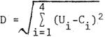
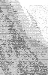 Figure 1 a raw image in band 5 of the multispectral scanner data. |
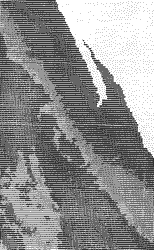 Figure 2. Classified imagery with different shades used to represent the various categories. |
 Figure 3. Same imagery as in figure 2, but with symbols chosen to highlight details along the border of the white portion of the imagery. | |