| GISdevelopment.net ---> AARS ---> ACRS 1980 ---> Technical Session |
Digital Processing of
Space-borne Synthetic Aperture Radar Data.
Histoshi Nohmi, Shiro Kato,
Nobuyasu Ito, Takenori Yanase
Hiromu Kashihara, Kenji Naito, Shinichi Hanaki
Nippon Electric Co.
Ltd., Tokyo Japan
Hiromu Kashihara, Kenji Naito, Shinichi Hanaki
Nippon Electric Co.
Ltd., Tokyo Japan
Abstract
This paper describes a digital processing for Synthetic Aperture Radar (SAR) imagery. SAR digital image processing consists of the following two parts. One is to compress the two dimensional hologram of terrain of earth. Another is to correct image distortion caused by altitude variations, velocity variations and altitude errors of platform, rotation of the earth, etc. As the image distortion could be compensated by Landsat technique, this paper deals with the technique of image reconstruction. In this paper, the Seasat SAR data are analized first, and then an example of image processing which was successfully accomplished for the first time in Japan is shown.
Introduction
Seasat is a marine observation satellite launched in 1978. It has Synthetic Aperture Radar (SAR), microwave radar altimeter, scatterometer and the other sensors. Recently, SAR has been remarked as a remote sensor for earth surface image because of its all-weather high resolution capability. SAR is a high resolution radar which obtains fine range and azimuth resolution by using pulse compression and synthetic aperture techniques. In SAR data processing, very large amount of operations are required to get image of earth surface. Optical processor with lens systems have been used to implement the large amount of operations. However, the development of digital processing system has been expected to take place of optical system because of flexibility, high accuracy and low distortions.
Seasat SAR Data
Seasat SAR system and its parameters are shown in Fig. 1 and Table 1 respectively. The SAR data to be processed are received at Oakhanger U.K. and include the information of about 100 Km x 100 Km area around the Lake of Leman and the Alps. The data are recorded in 6 magnetic tapes of 1600 BPI.

Fig 1 Seasat SAR System
| Radar Carrier Frequency | 1274.83 MHz |
| Pulse Repetition Frequency | 1646.67Hz |
| Pulse Duration | 33.9mS |
| FM Rate | 0.56 MHz/mS |
| Sampling Time | 21.97 nS |
The magnetic tape format consists of header files and data files. The header files have satellite position and velocity vectors data which are recorded every 60 seconds and attitude data recorded every 5 seconds. Some information in the header files are shown in Fig. 2,3 and 4. The SAR data digitalized to 5 bits consists of 13680 data records in range direction and 4096 data records in azimuth direction. Fig. 5 shows the frequency spectrum of the SAR data in range direction. It has high level components at the frequency of 11.38 MHz and 11.75MHz. These components seem to be caused by system noise and have to be eliminated in the data processing.
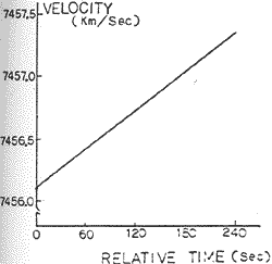 Fig 2 Velocity |
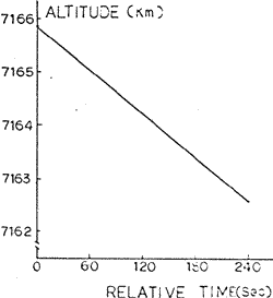 Fig 3 Altitude (From Earth Center) |
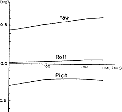 Fig 4 Time=0 is at 06: 42 GMT 19/8/'78. | |
SAR Data Processing
As shown in Fig. 6, the data processing can be divided into 5 steps. The programming was done principally in FORTRAN although assembly language coding was used to read SAR raw data. A general purpose computer, ACOS series 77/NEAC system 700 was used for this programming.
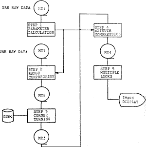
Block Diagram
Step 1 Parameter Calculation
After recording orbit and attitude data from the magnetic taps, parameters to be used in the following steps are calculated.
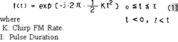
Step 2 Range Compression Range compression which compresses a chirp modulated signal to a sharp pulse in performed by correlating the SAR data with the reference function as shown in equation (1).
Convolution technique using the Fast Fourier Transform (FFT) in the frequency domain was adopted for saving CPU time in this compression.
Step 3 Corner Turning
Corner turning takes the data from the magnetic tape which is written in range line order, and rearranges it so that it can be read azimuth line order.
Step 4 Azimuth Compression
Modeling of the orbit is one of the important factors in the processing. In this processing system, Seasat orbit is regarded as an elliptic orbit as shown in Fig. 7. Assuming that time t= o when the relation between a target and the satellite satisfies the equation ( Rs x Vs ). R s x R t) = 0
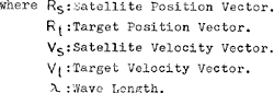
Doppler frequency can be written as follows
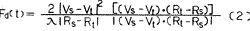
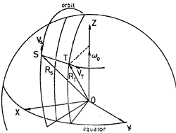
Coordinate System
Doppler frequency FD (t) spreads signal spectrum in azimuth direction as shown in Fig. 8 The power spectrum has an peak point at about –900Hz and approximately represents the Seasat antenna pattern. The peak point means the antenna beam center. Doppler frequency FD(t) is shown in Fig. 9 and can be represented by a linear function. The azimuth compression can only be done if the point target energy lies in a straight line in a signal memory which is so called “azimuth line” parallel to the azimuth axis. However, the point target energy lies in range lines as shown in Fig. 10.
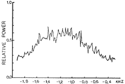
Example of Doppler Spectrum
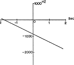
Doppler Frequency
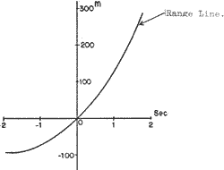
Range Curvature
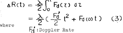
The variation of range between satellite and target ÑR is given as follows
Every target on the same range of line has the same functions of range curvature in the frequency domain. It is desirable to implement above compression after data have been transformed into the frequency domain. In the compensation, 4 points cubic convolution was adopted to reduce the effect of artifacts as shown in Fig. 11.
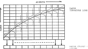
Rane Curvature Compensation.
A reference function for the azimuth compression is represented as a conjugate function of received signal from a point target. This function should be updated as range increases. It is updated when Doppler frequency of a target at the antenna beam center changes more than FFT resolution in this system. However, update rate could be reduced without degradation in image quality
In azimuth compression, the data spectrum is divided into 4 sub-spectrums, and independently reconstructed to 4 images.
Step 5 Multiple Looks
In multiple looks operation, 4 images get in step 4 are incoherently summed to reduce the special noise in SAR image called specle noise. This operation decreases resolution but increases the image quality because of reducing the noise. In summing of 4 images, image shift are required among them by a few pixcel in azimuth direction. This is because the reference function in azimuth compression is approximately to a linear function.
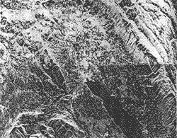
Seasat SAR Image
A SEASAT image through above steps in shown in Fig. 12. The image depict 50 Km x 40 Km area around Lake of Leman. Output data seem to have dynamic range of more than 30 dB. After operation of square root on the data, it is reduced to 18dB. The data is digitalized to 6 bit as a final image.
Conclusion
This paper described the digital processing steps of SAR raw data, first. Then, a high quality imaging of SEASAT data was shown to demonstrate the steps are valid. It is a subject for the authors to develop a high speed processing system based on above processing technique for future SAR system.
Reference
- (1) Lindt. W.J.: “Digital Technique for Generating Synthetic Aperture Radar Images”, IBM J. Res. Develop., p. 415 (Sept. 1977)
- A.B.E. Flles: “Ground Processing of Seasat-A SAR Data at an Enrthnet Station”. Proc. Internl. Conf. On Spacecraft Onboard Data Management, Nice, ESA-SP-141 (Dec. 1978) D.J. Bonfield, K.M. Harvey and J.R.E. Thomas “Synthetic Aperture Radar Real Time Processing”, Proc. Internl. Conf. On Spacecract on-board Data-Management, nice, ESA-SP-141 (Dec. 1978)
- Johne R. Bennett and Ian G. Cumming.: “Digital processor for The Production of Seasat Synthetic Aperture Radar Imagery”, Proc. Internl. Conf. On Seasat-SAR Processor, Frascati, ESA-SP-154 (Dec. 1979)
- Kirk, J.C.: “A Discussion of Digital Processing in Synthetic Aperture Radar”, IEEE Trons. Aerosp. Electron. Syst., AES-II, 3, P. 326 (May 1975)
- Bayma, R.W. at all.: “A Survey of SAR Image Formation Processing for Earth Resources Applications”, Proc. 11th Internatl. Symp. Remote Sensing of Environ., Michigan, P. 137 (Apr. 1977)
- Bennetti, J.R. and Cumming, I.G. “Digital SAR Image Formation Airborne and Satellite Results”, Proc. 13th Internatl. Symp. Remote Sensing of Environ., Michigan P. 337 (Apr. 1979)